Laboratory 4 - Estimation, filtering and system identification - Prof. M. Taragna
Exercise: Design of Kalman predictors and filters for a LTI dynamic system
Contents
Introduction
The program code may be splitted in sections using the characters "%%". Each section can run separately with the command "Run Section" (in the Editor toolbar, just to the right of the "Run" button). You can do the same thing by highlighting the code you want to run and by using the button function 9 (F9). This way, you can run only the desired section of your code, saving your time. This script can be considered as a reference example.
clear all, close all, clc
Procedure
- Load the file data.mat containing the input signal
- Define the LTI dynamic system S
- Define the noise variances
- Set the initial state of the LTI dynamic system S
- Simulate the LTI dynamic system S
- Plot states and output of the LTI dynamic system S
- Initialize the dynamic predictor K
- Simulate the dynamic predictor K and the filter F
- Compute the RMSEs for the dynamic predictor K and the filter F
- Plot the estimated states and output versus the actual ones
- Initialize the steady-state predictor Kinf
- Simulate the steady-state predictor Kinf and the filter Finf
- Compute the RMSEs for the steady-state predictor Kinf and the filter Finf
- Plot the estimated states and output versus the actual ones
- (Optional) Initialize the dynamic predictor Kpc
- (Optional) Simulate the dynamic predictor Kpc
Problem setup
% Step 1: load of data

load data
% u = input signal, computed as: sign(sin(2*pi*0.0005*(1:4000)))*1+10;

N=length(u); % N = number of data
N0_vector=[0, 20, 100];

% Step 2: definition of LTI dynamic system S

A=[ 0.96,  0.5,   0.27,  0.28; ...
   -0.125, 0.96, -0.08, -0.07; ...
    0,     0,     0.85,  0.97; ...
    0,     0,     0,     0.99];
B=[1; -1; 2; 1];
C=[0, 2, 0, 0];
D=[0];
% Note that: A is stable, (A,C) is observable

% Step 3: definition of noise variances

Bv1=sqrt(15)*[0.5; 0; 0; 1]; % Note that: (A,Bv1) is reachable
V1=Bv1*Bv1';
V2=2000;
V12=0;
rng('default'); % To produce the same random numbers at each run
LTI dynamic system simulation
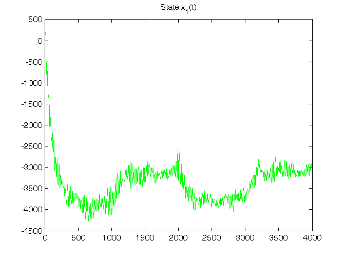
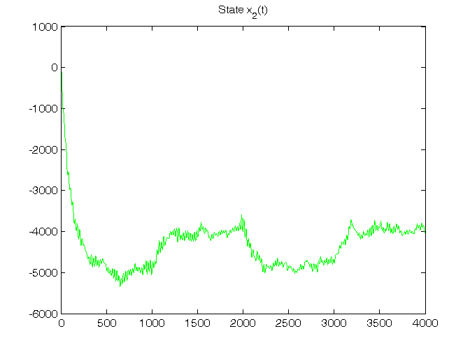
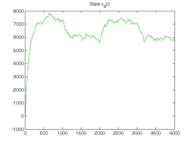
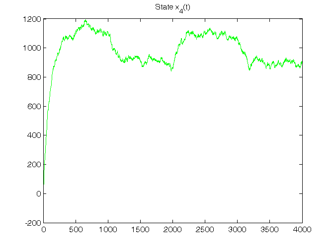
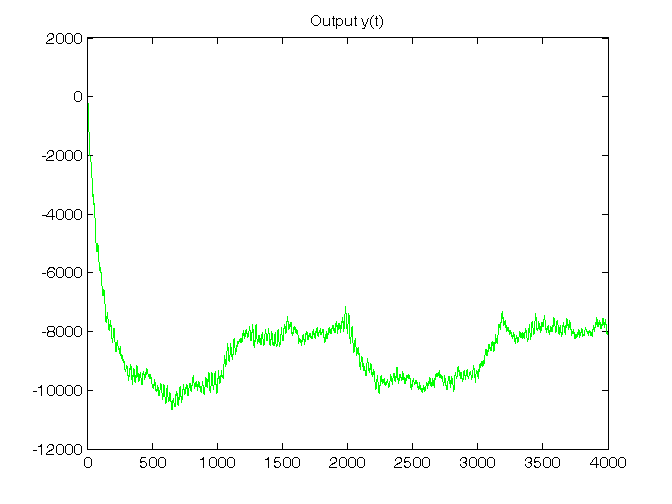
% Step 4: LTI dynamic system initialization

x(:,1)=[30; 40; -70; -10];
[n,nn]=size(A);

% Step 5: LTI dynamic system simulation

for t=1:N,

    % noises
    v1(:,t)=mvnrnd(zeros(1,n),Bv1*Bv1')';
    v2(t)=sqrt(V2)*randn;

    % system
    x(:,t+1)=A*x(:,t)+B*u(t)+v1(:,t);
    y(t)=C*x(:,t)+D*u(t)+v2(t);
end
Cov_v1=cov(v1'), V1 % To verify that: Var(v1) approximates V1
Cov_v2=cov(v2'), V2 % To verify that: Var(v2) approximates V2

% Step 6: plot of LTI system states and output

T=1:N;
for k=1:n,
    figure, plot(T,x(k,1:N),'g'), title(['State x_',num2str(k),'(t)'])
end
figure, plot(T,y(1:N),'g'), title('Output y(t)')
Cov_v1 =
    3.8177         0         0    7.6353
         0         0         0         0
         0         0         0         0
    7.6353         0         0   15.2707
V1 =
    3.7500         0         0    7.5000
         0         0         0         0
         0         0         0         0
    7.5000         0         0   15.0000
Cov_v2 =
   1.9130e+03
V2 =
        2000
Dynamic predictor K and filter F in standard form
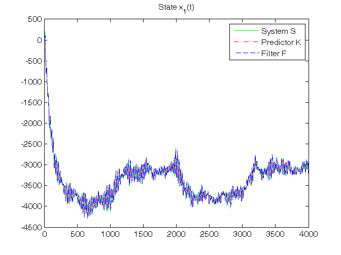
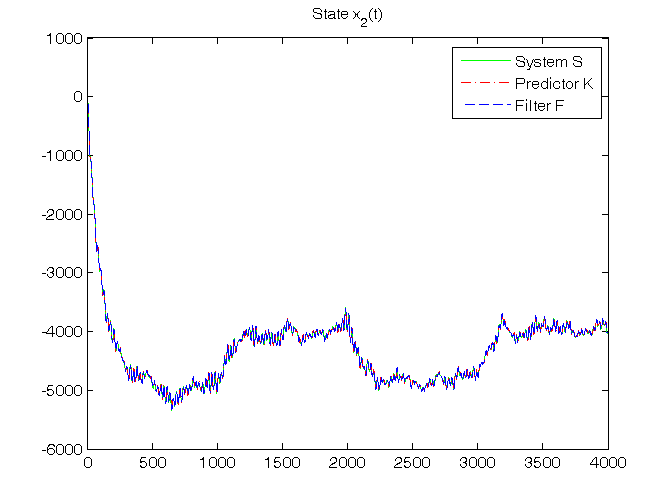
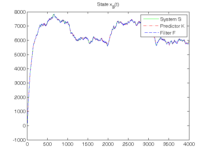
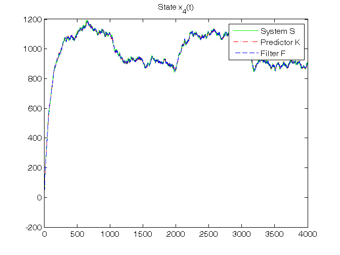
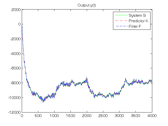
% Step 7: dynamic predictor K initialization

x_h(:,1)=zeros(n,1);
P{1}=0.5*eye(n);

% Step 8: dynamic predictor K and filter F simulation

for t=1:N,

    % dynamic predictor K
    y_h(t)=C*x_h(:,t);
    e(t)=y(t)-y_h(t);
    K{t}=(A*P{t}*C'+V12)*inv(C*P{t}*C'+V2);
    x_h(:,t+1)=A*x_h(:,t)+B*u(t)+K{t}*e(t);
    P{t+1}=A*P{t}*A'+V1-K{t}*(C*P{t}*C'+V2)*K{t}';

    % dynamic filter F
    K0{t}=P{t}*C'*inv(C*P{t}*C'+V2);
    x_f(:,t)=x_h(:,t)+K0{t}*e(t);
    y_f(t)=C*x_f(:,t);
end
K_N=K{N}
K0_N=K0{N}

% Step 9: RMSE computation

for ind=1:length(N0_vector),
    N0=N0_vector(ind);
    for k=1:n,
        RMSE_x_h(k,ind)=norm(x(k,N0+1:N)-x_h(k,N0+1:N))/sqrt(N-N0);
        RMSE_x_f(k,ind)=norm(x(k,N0+1:N)-x_f(k,N0+1:N))/sqrt(N-N0);
    end
    RMSE_y_h(ind)=norm(y(N0+1:N)-y_h(N0+1:N))/sqrt(N-N0);
    RMSE_y_f(ind)=norm(y(N0+1:N)-y_f(N0+1:N))/sqrt(N-N0);
end
fprintf('\n   N0 = %d    N0 = %d   N0 = %d\n',N0_vector(1),N0_vector(2),N0_vector(3))
RMSE_x_h, RMSE_y_h, RMSE_x_f, RMSE_y_f

% Step 10: graphical comparison of the results

for k=1:n,
    figure, plot(T,x(k,1:N),'g', T,x_h(k,1:N),'r-.', T,x_f(k,1:N),'b--'),
    title(['State x_',num2str(k),'(t)']), legend('System S','Predictor K','Filter F')
end
figure, plot(T,y(1:N),'g', T,y_h(1:N),'r-.', T,y_f(1:N),'b--'),
title('Output y(t)'), legend('System S','Predictor K','Filter F')
K_N =
   -0.2008
    0.2352
   -0.2881
   -0.0634
K0_N =
   -0.2148
    0.1902
   -0.2659
   -0.0640

   N0 = 0    N0 = 20   N0 = 100
RMSE_x_h =
   27.8311   27.5715   27.3745
   16.8500   16.7117   16.7443
   28.8517   28.7171   28.7069
   10.1058   10.0767   10.0442
RMSE_y_h =
   56.1359   55.7381   55.6878
RMSE_x_f =
   25.0575   24.7751   24.6337
   13.2025   13.0715   13.1061
   24.6422   24.5131   24.5315
    9.3866    9.3601    9.3394
RMSE_y_f =
   35.0983   34.5311   34.4994
Steady-state predictor Kinf and filter Finf in standard form
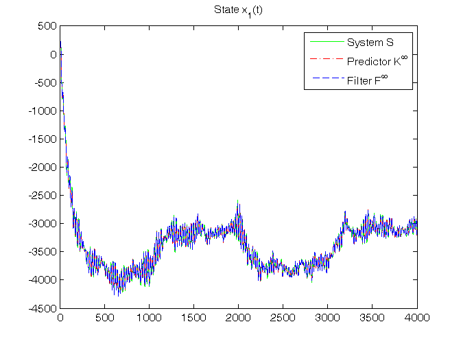
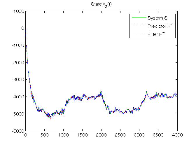
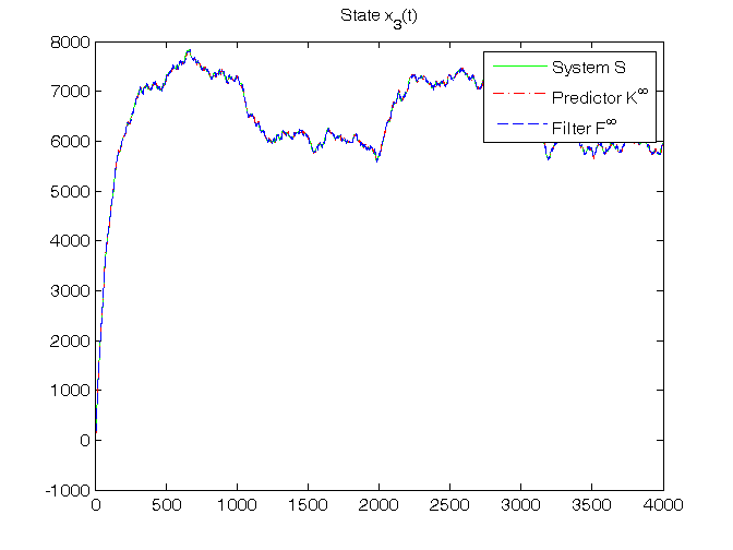
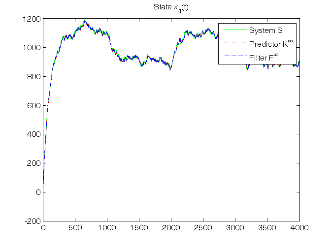
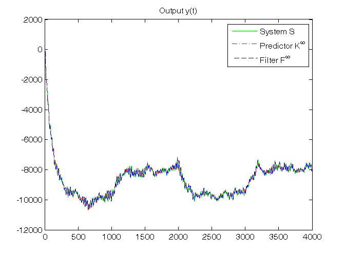
% Step 11: steady-state predictor Kinf initialization

x_h_ss(:,1)=zeros(n,1);

% Off-line computation of steady-state Kalman gain matrices
Sys1=ss(A,[B, eye(n)],C,[D, zeros(1,n)],1);
[Kalman_predictor,Kbar,Pbar,K0bar]=kalman(Sys1,V1,V2,0);
Kbar              % To verify that: Kbar  = K_N
K0bar             % To verify that: K0bar = K0_N
A_K0bar=A*K0bar   % To verify that: Kbar  = A*K0bar

% Step 12: steady-state predictor Kinf and filter Finf simulation

for t=1:N,

    % steady-state predictor Kinf
    y_h_ss(t)=C*x_h_ss(:,t);
    e_ss(t)=y(t)-y_h_ss(t);
    x_h_ss(:,t+1)=A*x_h_ss(:,t)+B*u(t)+Kbar*e_ss(t);

    % steady-state filter Finf
    x_f_ss(:,t)=x_h_ss(:,t)+K0bar*e_ss(t);
    y_f_ss(t)=C*x_f_ss(:,t);
end

% Step 13: RMSE computation

for ind=1:length(N0_vector),
    N0=N0_vector(ind);
    for k=1:n,
        RMSE_x_h_ss(k,ind)=norm(x(k,N0+1:N)-x_h_ss(k,N0+1:N))/sqrt(N-N0);
        RMSE_x_f_ss(k,ind)=norm(x(k,N0+1:N)-x_f_ss(k,N0+1:N))/sqrt(N-N0);
    end
    RMSE_y_h_ss(ind)=norm(y(N0+1:N)-y_h_ss(N0+1:N))/sqrt(N-N0);
    RMSE_y_f_ss(ind)=norm(y(N0+1:N)-y_f_ss(N0+1:N))/sqrt(N-N0);
end
fprintf('\n   N0 = %d    N0 = %d   N0 = %d\n',N0_vector(1),N0_vector(2),N0_vector(3))
RMSE_x_h_ss, RMSE_y_h_ss, RMSE_x_f_ss, RMSE_y_f_ss

% Step 14: graphical comparison of the results

for k=1:n,
    figure, plot(T,x(k,1:N),'g', T,x_h_ss(k,1:N),'r-.', T,x_f_ss(k,1:N),'b--'),
    title(['State x_',num2str(k),'(t)']), legend('System S','Predictor K^\infty','Filter F^\infty')
end
figure, plot(T,y(1:N),'g', T,y_h_ss(1:N),'r-.', T,y_f_ss(1:N),'b--'),
title('Output y(t)'), legend('System S','Predictor K^\infty','Filter F^\infty')
Kbar =
   -0.2008
    0.2352
   -0.2881
   -0.0634
K0bar =
   -0.2148
    0.1902
   -0.2659
   -0.0640
A_K0bar =
   -0.2008
    0.2352
   -0.2881
   -0.0634

   N0 = 0    N0 = 20   N0 = 100
RMSE_x_h_ss =
   27.6086   27.5865   27.3745
   16.7265   16.6999   16.7443
   28.7560   28.7026   28.7069
   10.0886   10.0766   10.0442
RMSE_y_h_ss =
   55.8566   55.7238   55.6878
RMSE_x_f_ss =
   24.8505   24.7931   24.6337
   13.0924   13.0657   13.1061
   24.5320   24.5037   24.5315
    9.3721    9.3600    9.3394
RMSE_y_f_ss =
   34.6039   34.5216   34.4994
(Optional) Dynamic predictor Kpc in predictor-corrector form
% Step 15: dynamic predictor Kpc initialization

x_h_pc(:,1)=zeros(n,1);
P{1}=0.5*eye(n);

% Step 16: dynamic predictor Kpc simulation

for t=1:N,
    K0{t}=P{t}*C'*inv(C*P{t}*C'+V2);
    P0{t}=(eye(n)-K0{t}*C)*P{t};
    P{t+1}=A*P0{t}*A'+V1;
    y_h_pc(t)=C*x_h_pc(:,t);
    e_pc(t)=y(t)-y_h_pc(t);
    x_f_pc(:,t)=x_h_pc(:,t)+K0{t}*e_pc(t);
    x_h_pc(:,t+1)=A*x_f_pc(:,t)+B*u(t);
end
norm(x_h-x_h_pc,inf) % To verify that: Kpc = K
norm(x_f-x_f_pc,inf) % To verify that: Fpc = F
ans =
   1.0246e-08
ans =
   9.3451e-09