Estimation, filtering and system identification - Prof. M. Taragna
Sample examination paper (exam duration: 3 hours)
Contents
- Introduction
- Problem #1.1-#1.2: Procedure
- Problem setup
- ARX identification, residual test and possible validation
- ARX comparison
- ARMAX identification, residual test and possible validation
- ARMAX comparison
- OE identification, residual test and possible validation
- OE comparison
- Trade-off selection between ARX/ARMAX/OE models
- Problem #1.3: Procedure
- Problem setup
- Evaluation of the Estimate Uncertainty Interval EUI_2
- Evaluation of the Parameter Uncertainty Interval PUI_2
- Evaluation of the Estimate Uncertainty Interval EUI_inf
Introduction
The program code may be splitted in sections using the characters "%%". Each section can run separately with the command "Run Section" (in the Editor toolbar, just to the right of the "Run" button). You can do the same thing by highlighting the code you want to run and by using the button function 9 (F9). This way, you can run only the desired section of your code, saving your time. This script can be considered as a reference example.
clear all, close all, clc
Problem #1.1-#1.2: Procedure
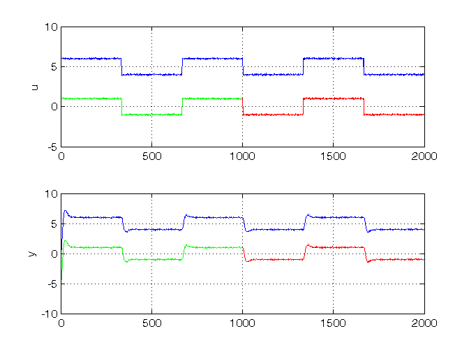
- Load the .mat file containing input-output data
- Remove the mean value from the data
- Plot input-output data
- Define estimation and validation datasets
- For each input-output delay nk from 1 to 3
- And for each order na=nb (ARX) / na=nb=nc (ARMAX) / nb=nf (OE) from 1 to 7
- Identify the ARX/ARMAX/OE model using the estimation dataset
- Perform the whiteness test on the estimation dataset
- Compute the predicted output on the validation dataset
- Compute the RMSE criterion
- Compare RMSE values
- Select the best trade-off between all the model classes
Problem setup
% Step 1: load of data

load('data1.mat')

% Step 2: remove the mean value

u_0mean = u - mean(u);
y_0mean = y - mean(y);

% Step 3: plot of input-output data

Ntot = length(u);
figure,
subplot(2,1,1), plot(1:Ntot,u), ylabel('u'), hold on;
subplot(2,1,2), plot(1:Ntot,y), ylabel('y'), hold on;

% Step 4: definition of estimation and validation datasets

Ne = Ntot/2;    % number of estimation data
Nv = Ntot - Ne; % number of validation data

ue = u_0mean(1:Ne);
uv = u_0mean(Ne+1:end);
ye = y_0mean(1:Ne);
yv = y_0mean(Ne+1:end);

DATAe = [ye,ue]; % estimation dataset
DATAv = [yv,uv]; % validation dataset

subplot(2,1,1), plot(1:Ne,ue,'g', Ne+1:Ntot,uv,'r'), grid on;
subplot(2,1,2), plot(1:Ne,ye,'g', Ne+1:Ntot,yv,'r'), grid on;
ARX identification, residual test and possible validation
To run this part in a smart way, you can put a break point at the command "close all" at the end of the external for-loop. This way you can check in figure k the corrisponding model with na=nb=k. After that you can click on "Continue" on the toolbar to evaluate for the next nk value. After the analysis you may comment the 'resid' command to speedup the next run instance.
% Step 5: loop on input-output delay

close all
for nk = 1:3,

    % Step 6: loop on model orders

    for k = 1:7,

        % Step 7: ARX(na=k,nb=k,nk) model identification

        na = k; nb = k;
        model = arx(DATAe,[na, nb, nk]);

        % Step 8: computation of model residuals and whiteness test

        % figure, resid(DATAe, model, 'corr', 30);

        % Step 9: computation of the predicted output on validation dataset

        yh = compare(DATAv, model, 1); % III param: 1 -> prediction; inf -> simulation

        % Step 10: RMSE computation on validation dataset

        N0 = 10;
        MSE = 1 /(Nv-N0)*norm(yv(N0+1:end)-yh(N0+1:end))^2;
        RMSE_arx(nk,k) = sqrt(MSE);
        n = na+nb;
        n_arx(k)=n;

    end
    close all
end
ARX comparison
The figures generated by resid show in the first part (AutoCorr) the residual values and the confidence intervals. You have to check all the generated plots: the more residual values are inside the confidence interval, the better is the model. You count the number of residuals sufficiently outside the confidence interval and you select a threshold: if this number is greater than the threshold, then the model is wasted, otherwise it is considered for further analysis. In this case, a reasonable threshold could be 3. The whiteness test results for ARX models are:
            na=1, na=2, na=3, na=4, na=5, na=6, na=7
       nk=1:   6     8     4     2     3     3     2
       nk=2:   6     8     4     2     3     3     2
       nk=3:   5     8     4     2     3     3     2
=> the ARX models that sufficiently satisfy the residual whiteness test are:
- For nk = 1, 2, 3: na = nb >= 4
Then the performance criteria can be printed
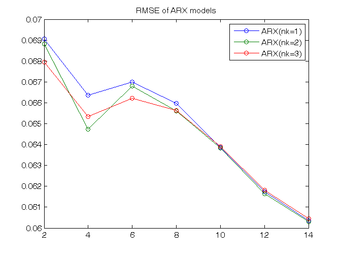
% Step 11: ARX comparison

RMSE_arx
figure, plot(n_arx,RMSE_arx','o-'), title('RMSE of ARX models'),
legend('ARX(nk=1)','ARX(nk=2)','ARX(nk=3)')

% The goal is to minimize the RMSE taking into account the previous
% residual test and the model complexity n, that for ARX models
% in prediction is n=na+nb
% The best trade-off between complexity and the validation criterion is
% the model ARX(4,4,2):

best_arx = arx(DATAe,[4,4,2]);
RMSE_arx442 = RMSE_arx(2,4)
RMSE_arx =
    0.0691    0.0664    0.0670    0.0660    0.0638    0.0617    0.0603
    0.0688    0.0647    0.0668    0.0656    0.0638    0.0617    0.0603
    0.0680    0.0653    0.0662    0.0656    0.0639    0.0618    0.0605
RMSE_arx442 =
    0.0656
ARMAX identification, residual test and possible validation
% Step 5: loop on input-output delay

close all
for nk = 1:3,

    % Step 6: loop on model orders

    for k = 1:7,

        % Step 7: ARMAX(na=k,nb=k,nc=k,nk) model identification

        na = k; nb = k; nc = k;
        model = armax(DATAe,[na, nb, nc, nk]);

        % Step 8: computation of model residuals and whiteness test

        % figure, resid(DATAe, model, 'corr', 30);

        % Step 9: computation of the predicted output on validation dataset

        yh = compare(DATAv, model, 1); % III param: 1 -> prediction; inf -> simulation

        % Step 10: RMSE computation on validation dataset

        N0 = 10;
        MSE = 1 /(Nv-N0)*norm(yv(N0+1:end)-yh(N0+1:end))^2;
        RMSE_armax(nk,k) = sqrt(MSE);
        n = na+nb+nc;
        n_armax(k)=n;

    end
    close all
end
ARMAX comparison
The whiteness test results for ARMAX models are:
            na=1, na=2, na=3, na=4, na=5, na=6, na=7
       nk=1:   5     0     0     0     0     0     0
       nk=2:   5     0     0     0     0     0     0
       nk=3:   6     0     0     0     0     0     0
=> the ARMAX models that sufficiently satisfy the residual whiteness test are:
- For nk = 1, 2, 3: na = nb = nc >= 2
Then the performance criteria can be printed
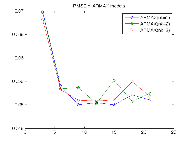
% Step 11: ARMAX comparison

RMSE_armax
figure, plot(n_armax,RMSE_armax','o-'), title('RMSE of ARMAX models'),
legend('ARMAX(nk=1)','ARMAX(nk=2)','ARMAX(nk=3)')

% The goal is to minimize the RMSE taking into account the previous
% residual test and the model complexity n, that for ARMAX models
% in prediction is n=na+nb+nc
% The best trade-off between complexity and the validation criterion is
% the model ARMAX(2,2,2,3):

best_armax = armax(DATAe,[2,2,2,3]);
RMSE_armax2223 = RMSE_armax(3,2)
RMSE_armax =
    0.0698    0.0540    0.0500    0.0504    0.0500    0.0521    0.0510
    0.0697    0.0534    0.0536    0.0502    0.0552    0.0508    0.0524
    0.0681    0.0532    0.0510    0.0508    0.0510    0.0549    0.0519
RMSE_armax2223 =
    0.0532
OE identification, residual test and possible validation
% Step 5: loop on input-output delay

close all
for nk = 1:3,

    % Step 6: loop on model orders

    for k = 1:7,

        % Step 7: OE(nb=k,nf=k,nk) model identification

        nb = k; nf = k;
        model = oe(DATAe,[nb, nf, nk]);

        % Step 8: computation of model residuals and whiteness test

        % figure, resid(DATAe, model, 'corr', 30);

        % Step 9: computation of the predicted output on validation dataset

        yh = compare(DATAv, model, 1); % III param: 1 -> prediction; inf -> simulation

        % Step 10: RMSE computation on validation dataset

        N0 = 10;
        MSE = 1 /(Nv-N0)*norm(yv(N0+1:end)-yh(N0+1:end))^2;
        RMSE_oe(nk,k) = sqrt(MSE);
        n = nb+nf;
        n_oe(k)=n;

    end
    close all
end
OE comparison
The whiteness test results for OE models are:
            nb=1, nb=2, nb=3, nb=4, nb=5, nb=6, nb=7
       nk=1:  14    10     0     0     0     0     0
       nk=2:  14    11     0     0     0     7     0
       nk=3:  13     5     0     0     0     8     0
=> the OE models that sufficiently satisfy the residual whiteness test are:
- For nk = 1: nb = nf >= 3
- For nk = 2, 3: nb = nf = 3, 4, 5, 7
Then the performance criteria can be printed
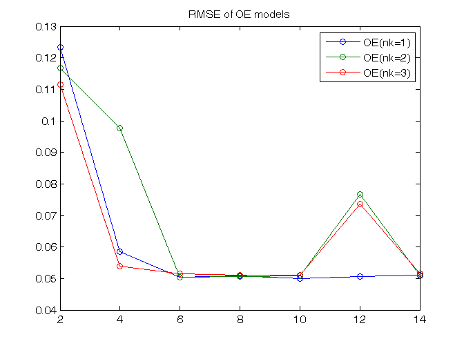
% Step 11: OE comparison

RMSE_oe
figure, plot(n_oe,RMSE_oe','o-'), title('RMSE of OE models'),
legend('OE(nk=1)','OE(nk=2)','OE(nk=3)')

% The goal is to minimize the RMSE taking into account the previous
% residual test and the model complexity n, that for OE models
% in prediction is n=nb+nf
% The best trade-off between complexity and the validation criterion is
% the model OE(3,3,1):

best_oe = oe(DATAe,[3,3,1]);
RMSE_oe331 = RMSE_oe(1,3)
RMSE_oe =
    0.1234    0.0584    0.0504    0.0507    0.0499    0.0507    0.0511
    0.1167    0.0976    0.0505    0.0506    0.0509    0.0766    0.0507
    0.1115    0.0538    0.0514    0.0511    0.0511    0.0737    0.0516
RMSE_oe331 =
    0.0504
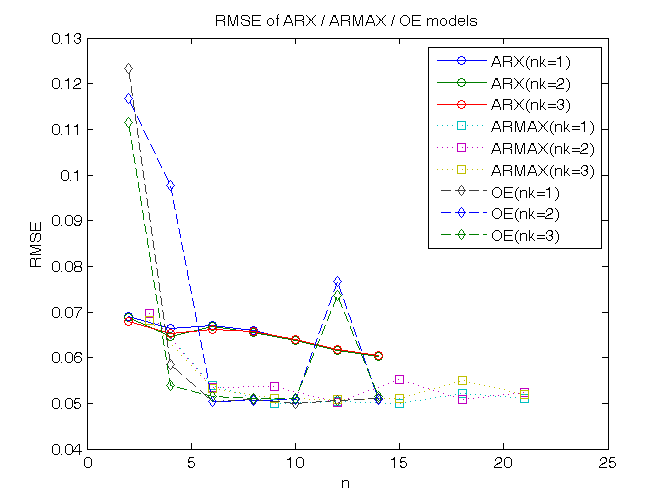
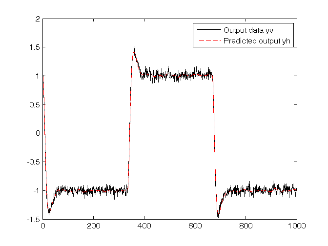
Trade-off selection between ARX/ARMAX/OE models
% Step 12: trade-off selection

% Graphical comparison of RMSE (to be minimized)
figure, plot(n_arx,RMSE_arx','o-',n_armax,RMSE_armax','s:',n_oe,RMSE_oe','d--'),
xlabel('n'), ylabel('RMSE'), title('RMSE of ARX / ARMAX / OE models'),
legend('ARX(nk=1)','ARX(nk=2)','ARX(nk=3)', ...
       'ARMAX(nk=1)','ARMAX(nk=2)','ARMAX(nk=3)','OE(nk=1)','OE(nk=2)','OE(nk=3)')

% The ARX(4,4,2) has higher complexity (n=8) and greater RMSE than the others.
% The ARMAX(2,2,2,3) and the OE(3,3,1) have the same complexity (n=6), but
% the RMSE value of the OE(3,3,1) is slightly lower (=> better)
%
% Conclusion: OE(3,3,1) is the best trade-off between performances and
% complexity.

best_tradeoff = oe(DATAe,[3,3,1]);
yh = compare(DATAv, best_tradeoff, 1); % III param: 1 -> prediction; inf -> simulation
figure, plot(1:Nv,yv,'-k',1:Nv,yh,'--r'),
legend('Output data yv','Predicted output yh');

present(best_tradeoff)
[A,B,C,D,F] = polydata(best_tradeoff)

% When used in prediction mode, the OE model transfer functions are:
% - between u(t) and yh(t): B(z)/F(z)
% - between y(t) and yh(t): 0
% Pay care that the polynomials B(z) and F(z) are in the z^-1 variable!!
best_tradeoff =
Discrete-time OE model:  y(t) = [B(z)/F(z)]u(t) + e(t)

  B(z) = 0.02393 (+/- 0.003342) z^-1 - 0.02032 (+/- 0.007383) z^-2
                                            - 0.002425 (+/- 0.004004) z^-3


  F(z) = 1 - 2.736 (+/- 0.01029) z^-1 + 2.504 (+/- 0.01923) z^-2 - 0.7665 (
                                                        +/- 0.009039) z^-3

Sample time: 1 seconds

Parameterization:
   Polynomial orders:   nb=3   nf=3   nk=1
   Number of free coefficients: 6
   Use "polydata", "getpvec", "getcov" for parameters and their uncertainties.

Status:
Termination condition: Near (local) minimum, (norm(g) < tol).
Number of iterations: 8, Number of function evaluations: 22

Estimated using OE on time domain data.
Fit to estimation data: 95.16%
FPE: 0.002655, MSE: 0.002625
More information in model's "Report" property.
A =
     1
B =
         0    0.0239   -0.0203   -0.0024
C =
     1
D =
     1
F =
    1.0000   -2.7360    2.5037   -0.7665
Problem #1.3: Procedure
- Estimate the parameters with the Least-squares algorithm
- Evaluate the Estimate Uncertainty Interval EUI_2
- Evaluate the Parameter Uncertainty Interval PUI_2 (if possible)
- Evaluate the Estimate Uncertainty Interval EUI_inf
Problem setup
The model ARX(3,3,1) can be parametrized with six parameters:
y(t) = -a1 y(t-1)-a2 y(t-2)-a3 y(t-3)+ b1 u(t-1)+b2 u(t-2)+b3 u(t-3)
Then the ARX parameters are estimated with the LS algorithm
% Step 1: Least-squares estimation

clear all, close all
load('data1.mat')
u = u - mean(u);
y = y - mean(y);
N = length(y);
PHI = [-y(3:N-1),-y(2:N-2),-y(1:N-3), u(3:N-1),u(2:N-2),u(1:N-3)];
Y = y(4:N);
theta = PHI\Y
theta =
   -0.6566
   -0.3219
    0.1074
    0.0195
    0.0328
    0.0832
Evaluation of the Estimate Uncertainty Interval EUI_2
The measurements are corrupted by an energy bounded noise whose 2-norm is less than 4. You can calculate the EUI_2 (see the official formulary)
% Step 2: evaluation of the Estimate Uncertainty Interval EUI_2

epsilon_2 = 4;
Sigma = inv(PHI'*PHI);
theta_min_2 = theta-epsilon_2*sqrt(diag(Sigma));
theta_max_2 = theta+epsilon_2*sqrt(diag(Sigma));
EUI_2=[theta_min_2, theta_max_2]
EUI_2 =
   -1.9391    0.6260
   -1.8080    1.1641
   -1.0511    1.2658
   -0.7246    0.7636
   -0.9347    1.0004
   -0.6985    0.8650
Evaluation of the Parameter Uncertainty Interval PUI_2
The measurements are corrupted by an energy bounded noise whose 2-norm is less than 4. Before to calculate the PUI_2, check if it is possibile: PUI_2 is not empty and can be computed only if alpha^2 <= epsilon_2^2
% Step 3: evaluation of the Parameter Uncertainty Interval PUI_2

alpha = norm(Y-PHI*theta)
if alpha^2 <= epsilon_2^2
   theta_min_2_ = theta-sqrt(diag(Sigma))*sqrt(epsilon_2^2-alpha^2);
   theta_max_2_ = theta+sqrt(diag(Sigma))*sqrt(epsilon_2^2-alpha^2);
   PUI_2 = [theta_min_2_, theta_max_2_]
end
alpha =
    3.0529
PUI_2 =
   -1.4853    0.1721
   -1.2821    0.6382
   -0.6411    0.8558
   -0.4613    0.5003
   -0.5924    0.6580
   -0.4219    0.5884
Evaluation of the Estimate Uncertainty Interval EUI_inf
The measurement error is bounded in magnitude by 0.1. You can calculate the EUI_inf
% Step 4: evaluation of the Estimate Uncertainty Interval EUI_inf

epsilon_inf = 0.1;
A = inv(PHI'*PHI)*PHI';
for ind=1:length(theta),
    theta_min_inf(ind,1)=A(ind,:)*(Y-epsilon_inf*sign(A(ind,:))');
    theta_max_inf(ind,1)=A(ind,:)*(Y+epsilon_inf*sign(A(ind,:))');
end
EUI_inf=[theta_min_inf, theta_max_inf]
EUI_inf =
   -1.7464    0.4332
   -1.6435    0.9996
   -0.8615    1.0762
   -0.3781    0.4171
   -0.5767    0.6423
   -0.3737    0.5402