Laboratory 6 - Estimation, filtering and system identification - Prof. M. Taragna
Exercise: model identification for a water heater, using linear models (real data)
Contents
Introduction
The program code may be splitted in sections using the characters "%%". Each section can run separately with the command "Run Section" (in the Editor toolbar, just to the right of the "Run" button). You can do the same thing by highlighting the code you want to run and by using the button function 9 (F9). This way, you can run only the desired section of your code, saving your time. This script can be considered as a reference example.
clear all, close all, clc
Procedure
- Load the .mat file containing input-output data
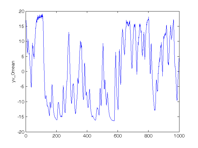
- Remove the mean value from the data
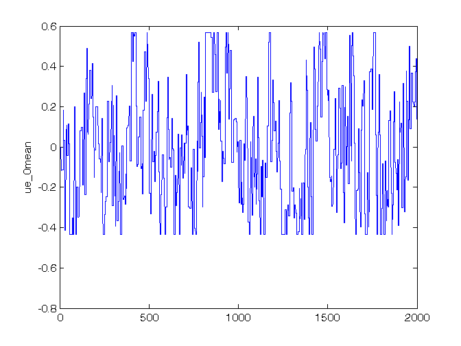
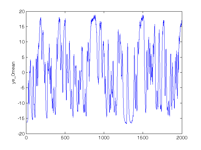
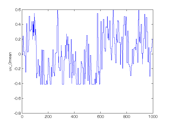
- Plot input-output data
- Define estimation and validation datasets
- For each input-output delay nk from 1 to 5
- And for each order na=nb (ARX) / nb=nf (OE) from 1 to 5
- Identify the ARX/OE model using the estimation dataset
- Perform the whiteness test on the estimation dataset
- Compute the predicted output on the validation dataset
- Compute the RMSE and MDL criteria
- Compare RMSE and MDL values
- Select the best trade-off between all the model classes
Problem setup
% Step 1: load of data

load heater

% Step 2: remove the mean value

ue_0mean = ue - mean(ue);
ye_0mean = ye - mean(ye);
uv_0mean = uv - mean(uv);
yv_0mean = yv - mean(yv);

% Step 3: plot of input-output data

Ne = length(ue); % number of estimation data
Nv = length(uv); % number of validation data

figure, plot(ue_0mean), ylabel('ue\_0mean'),
figure, plot(ye_0mean), ylabel('ye\_0mean'),
figure, plot(uv_0mean), ylabel('uv\_0mean'),
figure, plot(yv_0mean), ylabel('yv\_0mean')

% Step 4: definition of estimation and validation datasets

DATAe = [ye_0mean,ue_0mean]; % estimation dataset
DATAv = [yv_0mean,uv_0mean]; % validation dataset
ARX identification, residual test and possible validation
To run this part in a smart way, you can put a break point at the command "close all" at the end of the external for-loop. This way you can check in figure N the corrisponding model with na=nb=N. After that you can click on "Continue" on the toolbar to evaluate for the next nk value. After the analysis you may comment the 'resid' command to speedup the next run instance.
% Step 5: loop on input-output delay

close all
for nk = 1:5,

    % Step 6: loop on model orders

    for k = 1:5,

        % Step 7: ARX(na=k,nb=k,nk) model identification

        model = arx(DATAe,[k, k, nk]);

        % Step 8: computation of model residuals and whiteness test

        % figure, resid(DATAe, model, 'corr', 30);

        % Step 9: computation of the predicted output on validation dataset

        yh = compare(DATAv, model, 1); % III param: 1 -> prediction; inf -> simulation
        % figure, plot(1:Nv,yv_0mean,'-k',1:Nv,yh,'--r'),
        % title(['ARX(',num2str(k),',',num2str(k),',',num2str(nk),')']),
        % legend('Output data yv\_0mean','Predicted output yh');
        N0 = 10;

        % Step 10: RMSE and MDL computation on validation dataset

        MSE = 1 /(Nv-N0)*norm(yv_0mean(N0+1:end)-yh(N0+1:end))^2;
        RMSE_arx(nk,k) = sqrt(MSE);

        n = 2*k;
        n_arx(k)=n;
        MDL_arx(nk,k) = n*log(Nv-N0)/(Nv-N0)+log(MSE);

    end
    close all
end
ARX comparison
The figures generated by resid show in the first part (AutoCorr) the residual values and the confidence intervals. You have to check all the generated plots: the more residual values are inside the confidence interval, the better is the model. You count the number of residuals sufficiently outside the confidence interval and you select a threshold: if this number is greater than the threshold, then the model is wasted, otherwise it is considered for further analysis. In this case, a reasonable threshold could be 3. The whiteness test results for ARX models are:
            na=1, na=2, na=3, na=4, na=5
       nk=1:  10     2     2     1     2
       nk=2:  10     2     2     1     2
       nk=3:   7     2     1     1     1
       nk=4:   4     4     1     1     0
       nk=5:   5     3     1     0     1
=> the ARX models that sufficiently satisfy the residual whiteness test are:
- For nk = 1, 2, 3, 5: na = nb >= 2
- For nk = 4: na = nb >= 3
Then the performance criteria can be printed
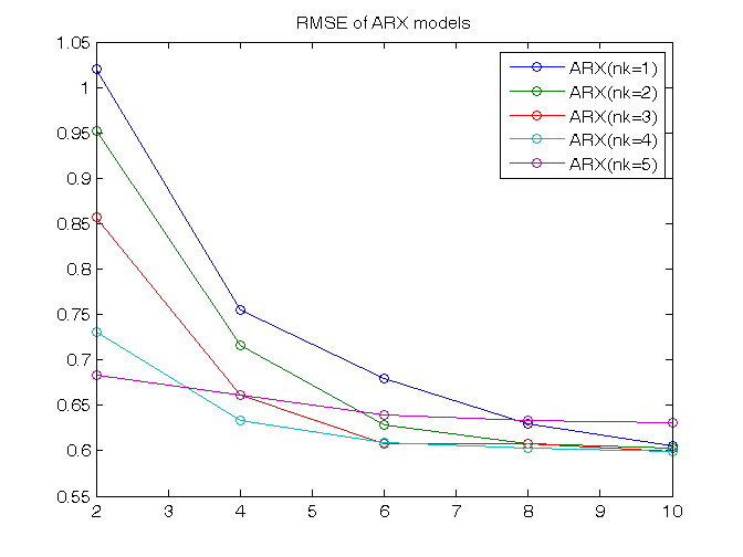
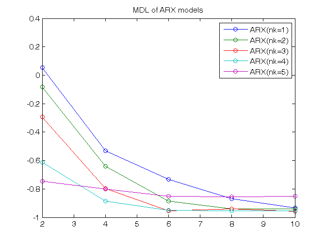
% Step 11: ARX comparison

RMSE_arx, MDL_arx
figure, plot(n_arx,RMSE_arx','o-'), title('RMSE of ARX models'),
legend('ARX(nk=1)','ARX(nk=2)','ARX(nk=3)','ARX(nk=4)','ARX(nk=5)')
figure, plot(n_arx,MDL_arx','o-'), title('MDL of ARX models'),
legend('ARX(nk=1)','ARX(nk=2)','ARX(nk=3)','ARX(nk=4)','ARX(nk=5)')
RMSE_arx =
    1.0199    0.7555    0.6790    0.6301    0.6054
    0.9524    0.7161    0.6286    0.6078    0.6035
    0.8569    0.6615    0.6077    0.6072    0.5988
    0.7309    0.6331    0.6088    0.6033    0.5996
    0.6836    0.6608    0.6394    0.6339    0.6313
MDL_arx =
    0.0533   -0.5330   -0.7325   -0.8680   -0.9340
   -0.0837   -0.6401   -0.8869   -0.9400   -0.9403
   -0.2949   -0.7985   -0.9544   -0.9420   -0.9559
   -0.6129   -0.8864   -0.9508   -0.9548   -0.9533
   -0.7468   -0.8008   -0.8525   -0.8559   -0.8502
OE identification, residual test and possible validation
% Step 5: loop on input-output delay

close all
for nk = 1:5,

    % Step 6: loop on model orders

    for k = 1:5,

        % Step 7: OE(nb=k,nf=k,nk) model identification

        model = oe(DATAe,[k, k, nk]);

        % Step 8: computation of model residuals and whiteness test

        % figure, resid(DATAe, model, 'corr', 30);

    end
    close all
end
OE comparison
The whiteness test results for OE models are:
            nb=1, nb=2, nb=3, nb=4, nb=5
      nk=1:   7    16    17    17    19
      nk=2:   7    16    17    17    14
      nk=3:  10    16    16    14    18
      nk=4:  14    16    16    18    17
      nk=5:  15    16    18    16    17
NO OE model passes the residual whiteness test with Threshold = 3 => OE is not the right model class in this case: for any order and delay, the number of residuals outside the confidence interval is too high
Trade-off selection
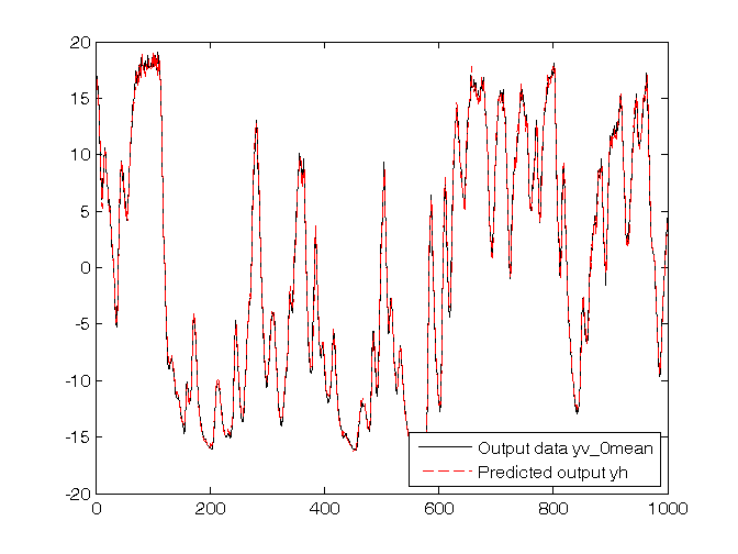
The goal is to minimize the RMSE and MDL criteria, taking into account the previous residual test and the model complexity n, that for models in prediction is: n=na+nb (ARX), n=nb+nf (OE) In this case, the ARX model class only has to be considered and the best trade-off between complexity and both the validation criteria is the ARX(3,3,3)
% Step 12: trade-off selection

best_tradeoff = arx(DATAe,[3,3,3]);
yh = compare(DATAv, best_tradeoff, 1); % III param: 1 -> prediction; inf -> simulation
figure, plot(1:Nv,yv_0mean,'-k',1:Nv,yh,'--r'),
legend('Output data yv\_0mean','Predicted output yh',4);

RMSE_best_tradeoff = RMSE_arx(3,3)
MDL_best_tradeoff = MDL_arx(3,3)

present(best_tradeoff)
[A,B,C,D,F] = polydata(best_tradeoff)

% When used in prediction mode, the ARX model transfer functions are:
% - between u(t) and yh(t): B(z)
% - between y(t) and yh(t): 1-A(z)
% Pay care that the polynomials A(z) and B(z) are in the z^-1 variable!!
RMSE_best_tradeoff =
    0.6077
MDL_best_tradeoff =
   -0.9544

best_tradeoff =
Discrete-time ARX model:  A(z)y(t) = B(z)u(t) + e(t)

  A(z) = 1 - 1.072 (+/- 0.02048) z^-1 - 0.09977 (+/- 0.03149) z^-2
                                               + 0.2512 (+/- 0.01675) z^-3


  B(z) = 0.3813 (+/- 0.1255) z^-3 + 1.468 (+/- 0.1734) z^-4 + 1.638 (
                                                          +/- 0.1552) z^-5

Sample time: 1 seconds

Parameterization:
   Polynomial orders:   na=3   nb=3   nk=3
   Number of free coefficients: 6
   Use "polydata", "getpvec", "getcov" for parameters and their uncertainties.

Status:
Estimated using ARX on time domain data.
Fit to estimation data: 93.69% (prediction focus)
FPE: 0.4125, MSE: 0.4112
More information in model's "Report" property.
A =
    1.0000   -1.0715   -0.0998    0.2512
B =
         0         0         0    0.3813    1.4678    1.6377
C =
     1
D =
     1
F =
     1