Laboratory 5 - Estimation, filtering and system identification - Prof. M. Taragna
Exercise 2: identification of a model for a dryer system
Contents
Introduction
The program code may be splitted in sections using the characters "%%". Each section can run separately with the command "Run Section" (in the Editor toolbar, just to the right of the "Run" button). You can do the same thing by highlighting the code you want to run and by using the button function 9 (F9). This way, you can run only the desired section of your code, saving your time. This script can be considered as a reference example.
clear all, close all, clc
Procedure
- Load the file dryer2.mat containing the input/output data
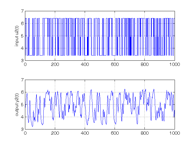
- Plot the input u2 and the output y2
- Remove the mean value from the data (with the function mean) in order to remove any systematic error
- Verify that it is correct with the function mean (it has to be zero)
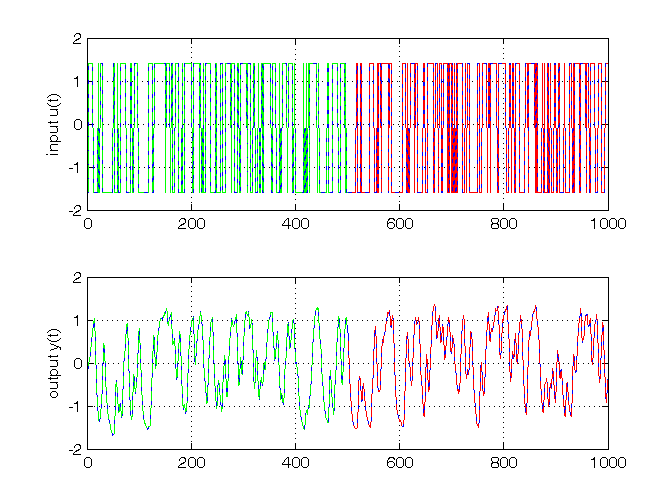
- Split the data in two parts: one for the parameter estimation and one for the model validation
- Define Ze and Zv as [ye,ue] and [yv,uv], respectively
- For each input/output delay nk from 1 to 4
- And for each order na=nb (ARX) / na=nb=nc (ARMAX) / nb=nf (OE) from 1 to 7
- Create the ARX/ARMAX/OE model with the function arx(Ze,[na,nb,nk]) / armax(Ze,[na,nb,nc,nk]) / oe(Ze,[nb,nf,nk])
- Perform the whiteness test with the resid(Ze,model,'CORR',30) function
- Compute the predicted output, with the compare(Zv,model,1) function, or the simulated output, with the compare(Zv,model,inf) function, and save it in yh
- Compute the criteria RMSE, FPE, etc... in order to select the most suitable model. You can find the formulas on the official formulary or on the slides.
Problem setup
% Step 1: load the data

load dryer2

% Step 2: plot the data

figure,
subplot(2,1,1), plot(u2), grid on, ylabel('input u2(t)')
subplot(2,1,2), plot(y2), grid on, ylabel('output y2(t)')

% Step 3: remove the mean values

u = u2 - mean(u2);
y = y2 - mean(y2);

% Step 4: verify the mean values of u and y

mean_u = mean(u)
mean_y = mean(y)

% Step 5: partition the data

Ntot = length(u);
Ne = Ntot/2;
Nv = Ntot-Ne;

ue = u(1:Ne);
uv = u(Ne+1:end);
ye = y(1:Ne);
yv = y(Ne+1:end);

figure,
subplot(2,1,1), plot(1:Ntot,u,'b', 1:Ne,ue,'g--', Ne+1:Ntot,uv,'r--'),
grid on, ylabel('input u(t)')
subplot(2,1,2), plot(1:Ntot,y,'b', 1:Ne,ye,'g--', Ne+1:Ntot,yv,'r--'),
grid on, ylabel('output y(t)')

% Step 6: define the datasets

Ze = [ye, ue]; % Estimation dataset
Zv = [yv, uv]; % Validation dataset
mean_u =
   7.2426e-14
mean_y =
  -7.1241e-15
ARX model class
To run this part in a smart way, you can put a break point at the command "close all" at the end of the external for-loop. This way you can check in figure N the corrisponding model with na=nb=N. After that you can click on "Continue" on the toolbar to evaluate for the next nk value. After the analysis you may comment the 'resid' command to speedup the next run instance.
close all
% Step 7
for nk = 1:4, % loop on the input-output delay
    % Step 8
    for na = 1:7, % loop on the order na
        nb = na;
        % Step 9: estimate the ARX parameters
        model = arx(Ze,[na,nb,nk]);

%         % Step 10: check the residual whiteness on the Estimation dataset
%         figure, resid(Ze,model,'CORR',30);

        % Step 11: compute the PREDICTED output on the Validation dataset
        yh = compare(Zv,model,1); % III param: 1 -> prediction; inf -> simulation
        % figure, plot(1:Nv,yv,'g', 1:Nv,yh,'r')

        % Step 12: compute the validation criteria
        N0 = 10;
        MSE = 1/(Nv-N0)*norm(yv(N0+1:end)-yh(N0+1:end))^2;
        n = na+nb; % model complexity for ARX models in prediction mode
        n_arx(na) = n;
        FPE_arx(nk,na) = (Nv-N0+n)/(Nv-N0-n)*MSE;
        AIC_arx(nk,na) = n*2/(Nv-N0)+log(MSE);
        MDL_arx(nk,na) = n*log(Nv-N0)/(Nv-N0)+log(MSE);
        FIT_arx(nk,na) = 1-sqrt(MSE/(1/(Nv-N0)*norm(yv(N0+1:end)-mean(yv(N0+1:end)))^2));
        if nk==3 & na==2, best_arx = model;  end
    end
%     pause, close all
end
The generated figures show in the first part (AutoCorr) the residual values and the confidence intervals. You have to check all the generated plots: the more residual values are inside the confidence interval, the better is the model. You count the number of residuals outside the confidence interval and you select a threshold: if this number is greater than the threshold, then the model is wasted, otherwise it is considered for further analyses. A reasonable threshold should be 4 or 5.
The models that sufficiently satisfy the residual whiteness test are:
- For nk = 1: na = nb >= 2
- For nk = 2, 3, 4: na = nb >= 1
Then you can print the performance criteria.
FPE_arx, AIC_arx, MDL_arx, FIT_arx
figure, plot(n_arx,FPE_arx(1,:),'r',n_arx,FPE_arx(2,:),'g',n_arx,FPE_arx(3,:),'b',n_arx,FPE_arx(4,:),'k'),
legend('nk = 1', 'nk = 2', 'nk = 3', 'nk = 4'), grid on, title('FPE for ARX models')
figure, plot(n_arx,AIC_arx(1,:),'r',n_arx,AIC_arx(2,:),'g',n_arx,AIC_arx(3,:),'b',n_arx,AIC_arx(4,:),'k'),
legend('nk = 1', 'nk = 2', 'nk = 3', 'nk = 4'), grid on, title('AIC for ARX models')
figure, plot(n_arx,MDL_arx(1,:),'r',n_arx,MDL_arx(2,:),'g',n_arx,MDL_arx(3,:),'b',n_arx,MDL_arx(4,:),'k'),
legend('nk = 1', 'nk = 2', 'nk = 3', 'nk = 4'), grid on, title('MDL for ARX models')
figure, plot(n_arx,FIT_arx(1,:),'r',n_arx,FIT_arx(2,:),'g',n_arx,FIT_arx(3,:),'b',n_arx,FIT_arx(4,:),'k'),
legend('nk = 1', 'nk = 2', 'nk = 3', 'nk = 4'), grid on, title('BEST FIT for ARX models')
FPE_arx =
    0.0378    0.0089    0.0025    0.0015    0.0014    0.0014    0.0014
    0.0313    0.0027    0.0015    0.0013    0.0013    0.0013    0.0014
    0.0146    0.0016    0.0014    0.0014    0.0014    0.0014    0.0014
    0.0113    0.0081    0.0082    0.0083    0.0084    0.0085    0.0086
AIC_arx =
   -3.2744   -4.7184   -6.0004   -6.5318   -6.6072   -6.5965   -6.5952
   -3.4656   -5.8963   -6.5067   -6.6083   -6.6110   -6.6104   -6.5917
   -4.2245   -6.4432   -6.5757   -6.5742   -6.5735   -6.5553   -6.5489
   -4.4866   -4.8204   -4.7980   -4.7918   -4.7842   -4.7644   -4.7603
MDL_arx =
   -3.2573   -4.6842   -5.9490   -6.4633   -6.5216   -6.4937   -6.4754
   -3.4485   -5.8621   -6.4553   -6.5398   -6.5254   -6.5076   -6.4719
   -4.2074   -6.4090   -6.5243   -6.5057   -6.4879   -6.4526   -6.4290
   -4.4695   -4.7862   -4.7467   -4.7233   -4.6986   -4.6617   -4.6404
FIT_arx =
    0.7630    0.8853    0.9398    0.9541    0.9560    0.9559    0.9560
    0.7846    0.9364    0.9533    0.9558    0.9560    0.9562    0.9560
    0.8526    0.9516    0.9549    0.9550    0.9552    0.9550    0.9550
    0.8707    0.8910    0.8903    0.8904    0.8904    0.8898    0.8900
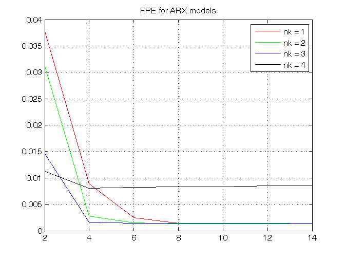
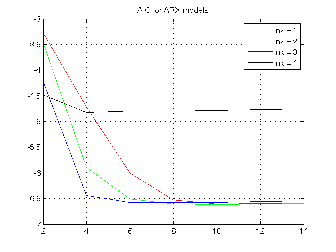
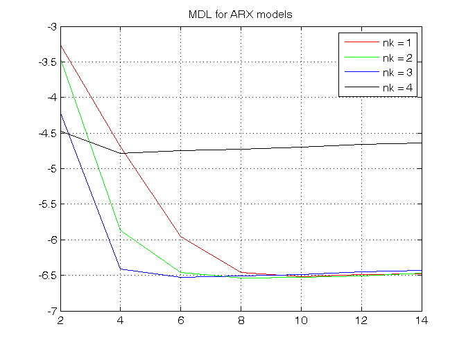
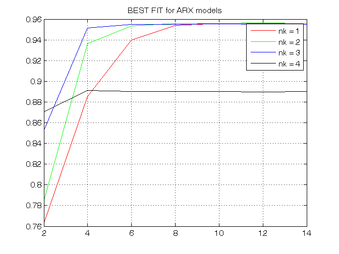
The goal is to minimize the criteria FPE, AIC and MDL and to maximize the best FIT, taking into account the complexity of the model, that for the ARX model is na+nb, and the previous residual test.
The best trade-off between complexity and any validation criterion is the model ARX(2,2,3):
present(best_arx)
[A,B,C,D,F] = polydata(best_arx);
A = tf(A,1,-1,'Variable','z^-1');
B = tf(B,1,-1,'Variable','z^-1');
TF_arx_pred_u = B
TF_arx_pred_y = 1-A
best_arx =
Discrete-time ARX model:  A(z)y(t) = B(z)u(t) + e(t)
  A(z) = 1 - 1.278 (+/- 0.01613) z^-1 + 0.3973 (+/- 0.01477) z^-2

  B(z) = 0.06518 (+/- 0.00163) z^-3 + 0.04497 (+/- 0.002492) z^-4

Sample time: 1 seconds

Parameterization:
   Polynomial orders:   na=2   nb=2   nk=3
   Number of free coefficients: 4
   Use "polydata", "getpvec", "getcov" for parameters and their uncertainties.

Status:
Estimated using ARX on time domain data.
Fit to estimation data: 95.06% (prediction focus)
FPE: 0.001728, MSE: 0.001714
More information in model's "Report" property.

TF_arx_pred_u =

  0.06518 z^-3 + 0.04497 z^-4

Sample time: unspecified
Discrete-time transfer function.


TF_arx_pred_y =

  1.278 z^-1 - 0.3973 z^-2

Sample time: unspecified
Discrete-time transfer function.
ARMAX model class
To run this part in a smart way, you can put a break point at the command "close all" at the end of the external for-loop. This way you can check in figure N the corrisponding model with na=nb=nc=N. After that you can click on "Continue" on the toolbar to evaluate for the next nk value. After the analysis you may comment the 'resid' command to speedup the next run instance.
close all
% Step 7
for nk = 1:4, % loop on the input-output delay
    % Step 8
    for na = 1:7, % loop on the order na
        nb = na;
        nc = na;
        % Step 9: estimate the ARMAX parameters
        model = armax(Ze,[na,nb,nc,nk]);

%         % Step 10: check the residual whiteness on the Estimation dataset
%         figure, resid(Ze,model,'CORR',30);

        % Step 11: compute the PREDICTED output on the Validation dataset
        yh = compare(Zv,model,1); % III param: 1 -> prediction; inf -> simulation
        % figure, plot(1:Nv,yv,'g', 1:Nv,yh,'r')

        % Step 12: compute the validation criteria
        N0 = 10;
        MSE = 1/(Nv-N0)*norm(yv(N0+1:end)-yh(N0+1:end))^2;
        n = na+nb+nc; % model complexity for ARMAX models in prediction mode
        n_armax(na) = n;
        FPE_armax(nk,na) = (Nv-N0+n)/(Nv-N0-n)*MSE;
        AIC_armax(nk,na) = n*2/(Nv-N0)+log(MSE);
        MDL_armax(nk,na) = n*log(Nv-N0)/(Nv-N0)+log(MSE);
        FIT_armax(nk,na) = 1-sqrt(MSE/(1/(Nv-N0)*norm(yv(N0+1:end)-mean(yv(N0+1:end)))^2));
        if nk==3 & na==2, best_armax = model; end
    end
%     pause, close all
end
The generated figures show in the first part (AutoCorr) the residual values and the confidence intervals. You have to check all the generated plots: the more residual values are inside the confidence interval, the better is the model. You count the number of residuals outside the confidence interval and you select a threshold: if this number is greater than the threshold, then the model is wasted, otherwise it is considered for further analyses. A reasonable threshold should be 4 or 5.
The models that sufficiently satisfy the residual whiteness test are:
- For nk = 1, 2, 3, 4: na = nb = nc >= 1
Then you can print the performance criteria.
FPE_armax, AIC_armax, MDL_armax, FIT_armax
figure, plot(n_armax,FPE_armax(1,:),'r',n_armax,FPE_armax(2,:),'g',n_armax,FPE_armax(3,:),'b',n_armax,FPE_armax(4,:),'k'),
legend('nk = 1', 'nk = 2', 'nk = 3', 'nk = 4'), grid on, title('FPE for ARMAX models')
figure, plot(n_armax,AIC_armax(1,:),'r',n_armax,AIC_armax(2,:),'g',n_armax,AIC_armax(3,:),'b',n_armax,AIC_armax(4,:),'k'),
legend('nk = 1', 'nk = 2', 'nk = 3', 'nk = 4'), grid on, title('AIC for ARMAX models')
figure, plot(n_armax,MDL_armax(1,:),'r',n_armax,MDL_armax(2,:),'g',n_armax,MDL_armax(3,:),'b',n_armax,MDL_armax(4,:),'k'),
legend('nk = 1', 'nk = 2', 'nk = 3', 'nk = 4'), grid on, title('MDL for ARMAX models')
figure, plot(n_armax,FIT_armax(1,:),'r',n_armax,FIT_armax(2,:),'g',n_armax,FIT_armax(3,:),'b',n_armax,FIT_armax(4,:),'k'),
legend('nk = 1', 'nk = 2', 'nk = 3', 'nk = 4'), grid on, title('BEST FIT for ARMAX models')
FPE_armax =
    0.0167    0.0073    0.0014    0.0014    0.0014    0.0015    0.0017
    0.0169    0.0023    0.0013    0.0013    0.0017    0.0016    0.0016
    0.0115    0.0014    0.0013    0.0013    0.0016    0.0017    0.0016
    0.0113    0.0082    0.0085    0.0090    0.0087    0.0090    0.0088
AIC_armax =
   -4.0921   -4.9234   -6.5493   -6.5950   -6.5688   -6.5016   -6.3680
   -4.0778   -6.0862   -6.6147   -6.6516   -6.3810   -6.4302   -6.4252
   -4.4626   -6.5681   -6.6142   -6.6127   -6.4158   -6.3718   -6.4189
   -4.4829   -4.8000   -4.7683   -4.7138   -4.7426   -4.7141   -4.7305
MDL_armax =
   -4.0664   -4.8720   -6.4722   -6.4923   -6.4404   -6.3475   -6.1882
   -4.0521   -6.0348   -6.5377   -6.5489   -6.2526   -6.2761   -6.2454
   -4.4369   -6.5167   -6.5371   -6.5100   -6.2874   -6.2177   -6.2391
   -4.4572   -4.7486   -4.6913   -4.6110   -4.6142   -4.5600   -4.5507
FIT_armax =
    0.8429    0.8969    0.9546    0.9559    0.9556    0.9543    0.9515
    0.8417    0.9424    0.9560    0.9571    0.9512    0.9527    0.9528
    0.8694    0.9547    0.9560    0.9563    0.9520    0.9513    0.9527
    0.8708    0.8904    0.8893    0.8869    0.8892    0.8883    0.8899
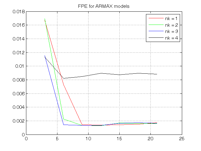
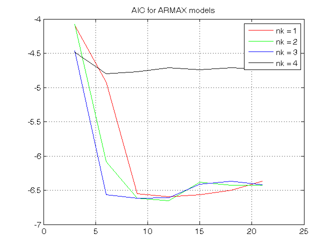
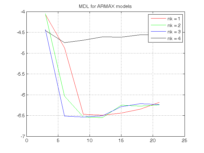
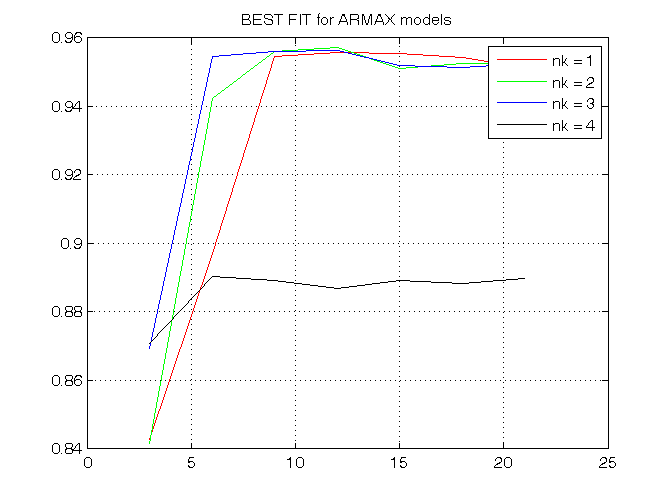
The goal is to minimize the criteria FPE, AIC and MDL and to maximize the best FIT, taking into account the complexity of the model, that for the ARMAX model is na+nb+nc, and the previous residual test.
The best trade-off between complexity and any validation criterion is the model ARXMAX(2,2,2,3):
present(best_armax)
[A,B,C,D,F] = polydata(best_armax)
A = tf(A,1,-1,'Variable','z^-1');
B = tf(B,1,-1,'Variable','z^-1');
C = tf(C,1,-1,'Variable','z^-1');
TF_armax_pred_u = B/C
TF_armax_pred_y = 1-A/C
best_armax =
Discrete-time ARMAX model:  A(z)y(t) = B(z)u(t) + C(z)e(t)
  A(z) = 1 - 1.309 (+/- 0.01441) z^-1 + 0.4255 (+/- 0.01302) z^-2

  B(z) = 0.06578 (+/- 0.001562) z^-3 + 0.04122 (+/- 0.002603) z^-4

  C(z) = 1 - 0.3403 (+/- 0.04806) z^-1 + 0.1125 (+/- 0.04542) z^-2

Sample time: 1 seconds

Parameterization:
   Polynomial orders:   na=2   nb=2   nc=2   nk=3
   Number of free coefficients: 6
   Use "polydata", "getpvec", "getcov" for parameters and their uncertainties.

Status:
Termination condition: Near (local) minimum, (norm(g) < tol).
Number of iterations: 5, Number of function evaluations: 11

Estimated using ARMAX on time domain data.
Fit to estimation data: 95.23% (prediction focus)
FPE: 0.00166, MSE: 0.001601
More information in model's "Report" property.
A =
    1.0000   -1.3086    0.4255
B =
         0         0         0    0.0658    0.0412
C =
    1.0000   -0.3403    0.1125
D =
     1
F =
     1

TF_armax_pred_u =

   0.06578 z^-3 + 0.04122 z^-4
  -----------------------------
  1 - 0.3403 z^-1 + 0.1125 z^-2

Sample time: unspecified
Discrete-time transfer function.


TF_armax_pred_y =

    0.9682 z^-1 - 0.313 z^-2
  -----------------------------
  1 - 0.3403 z^-1 + 0.1125 z^-2

Sample time: unspecified
Discrete-time transfer function.
OE model class
To run this part in a smart way, you can put a break point at the command "close all" at the end of the external for-loop. This way you can check in figure N the corrisponding model with nb=nf=N. After that you can click on "Continue" on the toolbar to evaluate for the next nk value. After the analysis you may comment the 'resid' command to speedup the next run instance.
close all
% Step 7
for nk = 1:4, % loop on the input-output delay
    % Step 8
    for nf = 1:7, % loop on the order nf
        nb = nf;
        % Step 9: estimate the OE parameters
        model = oe(Ze, [nb,nf,nk]);

%         % Step 10: check the residual whiteness on the Estimation dataset
%         figure, resid(Ze, model, 'CORR', 30');

        % Step 11: compute the PREDICTED output on the Validation dataset
        yh = compare(Zv,model,1); % III param: 1 -> prediction; inf -> simulation
        % figure, plot(1:Nv,yv,'g', 1:Nv,yh,'r')

        % Step 12: compute the validation criteria
        N0 = 10;
        MSE=1/(Nv-N0)*norm(yv(N0+1:end)-yh(N0+1:end))^2;
        n = nb+nf; % model complexity for OE models in prediction mode
        n_oe(nf) = n;
        FPE_oe(nk,nf) = (Nv-N0+n)/(Nv-N0-n)*MSE;
        AIC_oe(nk,nf) = n*2/(Nv-N0)+log(MSE);
        MDL_oe(nk,nf) = n*log(Nv-N0)/(Nv-N0)+log(MSE);
        FIT_oe(nk,nf) = 1-sqrt(MSE/(1/(Nv-N0)*norm(yv(N0+1:end)-mean(yv(N0+1:end)))^2));
    end
%     pause, close all
end
The generated figures show in the first part (AutoCorr) the residual values and the confidence intervals. You have to check all the generated plots: the more residual values are inside the confidence interval, the better is the model. You count the number of residuals outside the confidence interval and you select a threshold: if this number is greater than the threshold, then the model is wasted, otherwise it is considered for further analyses. A reasonable threshold should be 4 or 5.
The models that sufficiently satisfy the residual whiteness test are:
- For nk = 2, 3: na = nb = nc = 1
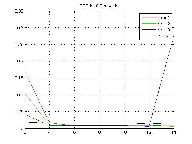
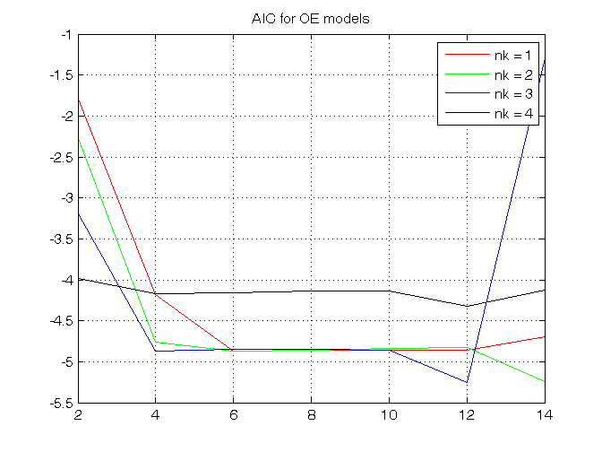
OE is not a good model class for this example: for almost all the orders, the number of residuals outside the confidence interval is high.
Then you can print the performance criteria.
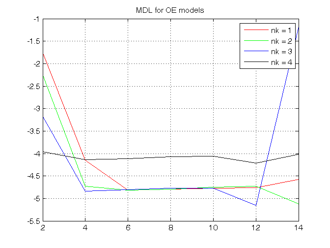
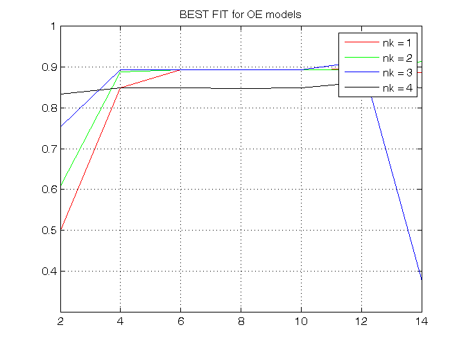
FPE_oe, AIC_oe, MDL_oe, FIT_oe
figure, plot(n_oe,FPE_oe(1,:),'r',n_oe,FPE_oe(2,:),'g',n_oe,FPE_oe(3,:),'b',n_oe,FPE_oe(4,:),'k'),
legend('nk = 1', 'nk = 2', 'nk = 3', 'nk = 4'), grid on, title('FPE for OE models')
figure, plot(n_oe,AIC_oe(1,:),'r',n_oe,AIC_oe(2,:),'g',n_oe,AIC_oe(3,:),'b',n_oe,AIC_oe(4,:),'k'),
legend('nk = 1', 'nk = 2', 'nk = 3', 'nk = 4'), grid on, title('AIC for OE models')
figure, plot(n_oe,MDL_oe(1,:),'r',n_oe,MDL_oe(2,:),'g',n_oe,MDL_oe(3,:),'b',n_oe,MDL_oe(4,:),'k'),
legend('nk = 1', 'nk = 2', 'nk = 3', 'nk = 4'), grid on, title('MDL for OE models')
figure, plot(n_oe,FIT_oe(1,:),'r',n_oe,FIT_oe(2,:),'g',n_oe,FIT_oe(3,:),'b',n_oe,FIT_oe(4,:),'k'),
legend('nk = 1', 'nk = 2', 'nk = 3', 'nk = 4'), grid on, title('BEST FIT for OE models')
FPE_oe =
    0.1693    0.0153    0.0077    0.0077    0.0078    0.0078    0.0092
    0.1037    0.0085    0.0077    0.0077    0.0079    0.0080    0.0053
    0.0413    0.0077    0.0078    0.0079    0.0078    0.0052    0.2756
    0.0187    0.0154    0.0156    0.0159    0.0159    0.0133    0.0161
AIC_oe =
   -1.7764   -4.1771   -4.8669   -4.8643   -4.8560   -4.8596   -4.6924
   -2.2660   -4.7643   -4.8701   -4.8617   -4.8367   -4.8284   -5.2434
   -3.1877   -4.8678   -4.8524   -4.8446   -4.8571   -5.2552   -1.2886
   -3.9780   -4.1720   -4.1635   -4.1418   -4.1417   -4.3194   -4.1308
MDL_oe =
   -1.7593   -4.1429   -4.8155   -4.7958   -4.7704   -4.7569   -4.5725
   -2.2489   -4.7301   -4.8188   -4.7932   -4.7511   -4.7257   -5.1236
   -3.1706   -4.8336   -4.8010   -4.7761   -4.7715   -5.1525   -1.1688
   -3.9609   -4.1378   -4.1121   -4.0734   -4.0561   -4.2167   -4.0110
FIT_oe =
    0.4988    0.8497    0.8940    0.8943    0.8943    0.8949    0.8862
    0.6076    0.8880    0.8942    0.8941    0.8932    0.8932    0.9136
    0.7525    0.8936    0.8932    0.8932    0.8943    0.9138    0.3759
    0.8333    0.8493    0.8493    0.8483    0.8489    0.8623    0.8493
Choosing the best model
FPE (to be minimized)
FPE_arx(3,2)
FPE_armax(3,2)
ans =
    0.0016
ans =
    0.0014
ARMAX(2,2,2,3) has slightly better performance but much higher complexity than ARX(2,2,3)
AIC (to be minimized)
AIC_arx(3,2)
AIC_armax(3,2)
ans =
   -6.4432
ans =
   -6.5681
ARMAX(2,2,2,3) has slightly better performance but much higher complexity than ARX(2,2,3)
MDL (to be minimized)
MDL_arx(3,2)
MDL_armax(3,2)
ans =
   -6.4090
ans =
   -6.5167
ARMAX(2,2,2,3) has slightly better performance but much higher complexity than ARX(2,2,3)
FIT (to be maximized)
FIT_arx(3,2)
FIT_armax(3,2)
ans =
    0.9516
ans =
    0.9547
ARMAX(2,2,2,3) has slightly better performance but much higher complexity than ARX(2,2,3)
Conclusion: ARX(2,2,3) is the best trade-off between performances and complexity