Laboratory 5 - Estimation, filtering and system identification - Prof. M. Taragna
Exercise 1: parameter convergence in ARX model identification (simulated data)
Contents
Introduction
The program code may be splitted in sections using the characters "%%". Each section can run separately with the command "Run Section" (in the Editor toolbar, just to the right of the "Run" button). You can do the same thing by highlighting the code you want to run and by using the button function 9 (F9). This way, you can run only the desired section of your code, saving your time. This script can be considered as a reference example.
clear all, close all, clc
Procedure
- Define the ARX parameters
- Compute the ARX output
- Plot the ARX output
- Estimate the ARX parameters using the Least Squares algorithm
- Plot the estimated parameters versus the actual parameters
- Compute the prediction error using the final estimated parameters
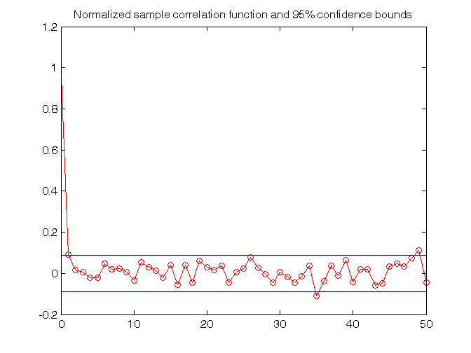
- Perform the Anderson's whiteness test using the xcorr function
Problem setup
% Step 1: definition of ARX parameters

a1=0.93;
b1=1.5;
b2=-3;
theta0=[a1;b1;b2]
theta0 =
    0.9300
    1.5000
   -3.0000
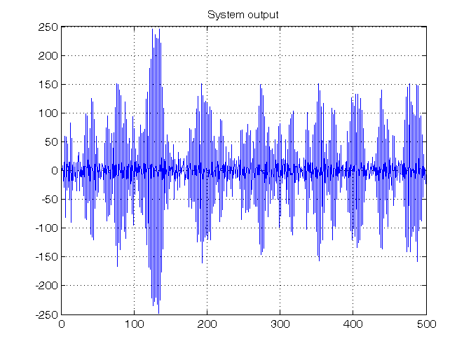
System simulation
% Step 2: computation of ARX output

Nmax=500;
rng('default')
u=10*(-1+2*rand(Nmax,1));

for t=1:Nmax,
   d(t)=3*randn;
   if t==1,
      phi(:,t)=[0; 0; 0];
   elseif t==2,
      phi(:,t)=[-y(t-1); u(t-1); 0];
   else
      phi(:,t)=[-y(t-1); u(t-1); u(t-2)];
   end
   y(t,1)=phi(:,t)'*theta0+d(t);
end

% Step 3: plot of ARX output

figure,
plot(y), grid on, title('System output')
System identification
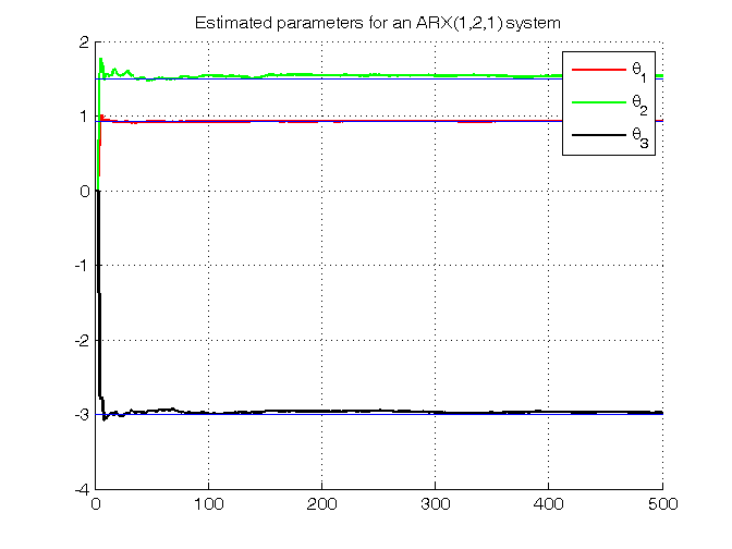
% Step 4: computation of the parameter estimates using Least Squares

Phi=[];
R_toll=1e-10;
for t=1:Nmax,
    if t==1,
       phi(:,t)=[0; 0; 0];
    elseif t==2,
       phi(:,t)=[-y(t-1); u(t-1); 0];
    else
       phi(:,t)=[-y(t-1); u(t-1); u(t-2)];
    end
    Phi=[Phi; phi(:,t)'];
    Y=y(1:t);
    R_t=Phi'*Phi/t;
    if abs(det(R_t))>R_toll,
       theta_t1(:,t)=inv(R_t)*(Phi'/t)*Y;
       theta_t2(:,t)=pinv(Phi)*Y;
       theta_t3(:,t)=Phi\Y;
    else
       theta_t1(:,t)=zeros(size(theta0));
       theta_t2(:,t)=zeros(size(theta0));
       theta_t3(:,t)=zeros(size(theta0));
    end
end
theta_Nmax=theta_t1(:,Nmax)

% Numerical comparison of results
norm(theta_t1-theta_t2,inf)
norm(theta_t1-theta_t3,inf)
norm(theta_t2-theta_t3,inf)

% Step 5: graphical comparison of the results

figure, hold on
plot(theta_t1(1,:),'r','LineWidth',1.5)
plot(theta_t1(2,:),'g','LineWidth',1.5)
plot(theta_t1(3,:),'k','LineWidth',1.5)
for ind=1:length(theta0),
    refline(0,theta0(ind))
end
grid on, title('Estimated parameters for an ARX(1,2,1) system')
legend('\theta_1','\theta_2','\theta_3')
theta_Nmax =
    0.9293
    1.5350
   -2.9793
ans =
   1.0352e-12
ans =
   6.9234e-13
ans =
   9.8832e-13
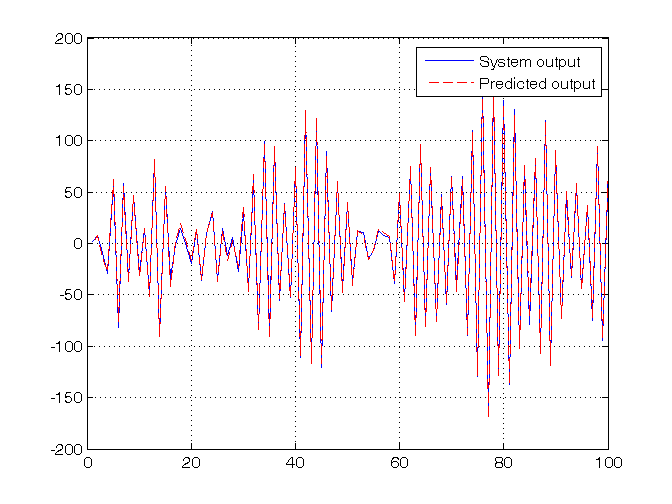
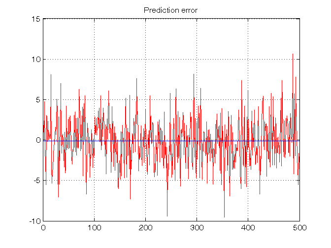
System validation
% Step 6: computation of the prediction error for the final estimates

for t=1:Nmax,
    if t==1,
       phi(:,t)=[0; 0; 0];
    elseif t==2,
       phi(:,t)=[-y(t-1); u(t-1); 0];
    else
       phi(:,t)=[-y(t-1); u(t-1); u(t-2)];
    end
    y_hat(t,1)=phi(:,t)'*theta_Nmax;
end
pred_error=y-y_hat;
pred_error_mean=mean(pred_error)

figure,
plot(1:Nmax,y,'b', 1:Nmax,y_hat,'r--'), grid on, xlim([0, 100])
legend('System output', 'Predicted output')

figure,
plot(pred_error,'r'), grid on, title('Prediction error')
refline(0,pred_error_mean)

% Step 7: computation of the normalized sample correlation function

[r,lags] = xcorr(pred_error,'coeff');
figure, plot(lags,r,'ro-'), xlim([0, 50]),
refline(0,2/sqrt(Nmax)), refline(0,-2/sqrt(Nmax)), % 95% confidence bounds
title('Normalized sample correlation function and 95% confidence bounds')
pred_error_mean =
   -0.1379