Laboratory 3 - Estimation, filtering and system identification - Prof. M. Taragna
Exercise 2: Parametric estimation of an auto-regressive model from output data
Contents
Introduction
The program code may be splitted in sections using the characters "%%". Each section can run separately with the command "Run Section" (in the Editor toolbar, just to the right of the "Run" button). You can do the same thing by highlighting the code you want to run and by using the button function 9 (F9). This way, you can run only the desired section of your code, saving your time. This script can be considered as a reference example.
clear all, close all, clc
Procedure
- Load the file AR_data.mat containing the output data
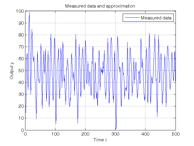
- Plot the experimental data
- Estimate the model parameters using the Least Squares algorithm
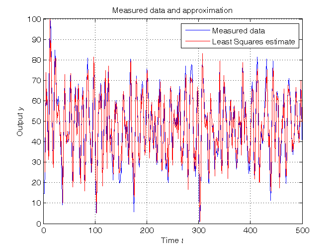
- Plot the estimated approximation versus the experimental data
Problem setup
% Step 1: load of data

load AR_data.mat
% y = output samples

L = length(y); % L = number of data

% Step 2: plot of data

figure, plot(1:L,y,'-b'),
axis([0,L,0,100]), grid, title('Measured data and approximation'),
xlabel('Time{\it t}'), ylabel('Output{\it y}'),
legend('Measured data',1)
Estimation of the model parameters using the Least Squares algorithm
% Step 3: computation of the parameter estimate

Y=y(3:L);
Phi=[-y(2:L-1), -y(1:L-2), ones(L-2,1)];
theta_LS=Phi\Y % Form #1: using the "\" operator (more realiable)

A=pinv(Phi);   % more realiable than inv(Phi'*Phi)*Phi'
theta_LS_=A*Y  % Form #2: using the pseudoinverse matrix
a1=theta_LS(1)
a2=theta_LS(2)
b=theta_LS(3)

sigma_e=sqrt(40);
Sigma_theta=sigma_e^2*inv(Phi'*Phi) % Variance matrix of the estimates
sigma_theta=sqrt(diag(Sigma_theta)) % Standard deviations of the estimates

% Step 4: graphical comparison of the results

y_LS = Phi*theta_LS;
figure, plot(1:L,y,'-b', 3:L,y_LS,'-r'),
axis([0,L,0,100]), grid, title('Measured data and approximation'),
xlabel('Time{\it t}'), ylabel('Output{\it y}'),
legend('Measured data','Least Squares estimate',1)
theta_LS =
   -1.4301
    0.7488
   15.1412
theta_LS_ =
   -1.4301
    0.7488
   15.1412
a1 =
   -1.4301
a2 =
    0.7488
b =
   15.1412
Sigma_theta =
    0.0009   -0.0007    0.0078
   -0.0007    0.0009    0.0073
    0.0078    0.0073    0.7979
sigma_theta =
    0.0297
    0.0296
    0.8932