Laboratory 3 - Estimation, filtering and system identification - Prof. M. Taragna
Exercise 1: Parametric estimation of a resistance from current-voltage data stored in resistor_data_1.mat
Contents
Introduction
The program code may be splitted in sections using the characters "%%". Each section can run separately with the command "Run Section" (in the Editor toolbar, just to the right of the "Run" button). You can do the same thing by highlighting the code you want to run and by using the button function 9 (F9). This way, you can run only the desired section of your code, saving your time. This script can be considered as a reference example.
clear all, close all, clc
Procedure
- Load the file resistor_data_1.mat containing the current-voltage data
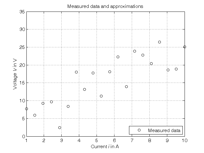
- Plot the voltage measurements versus the current measurements
- Estimate the resistance using the Sample Mean algorithm
- Plot the estimated approximation versus the experimental data
- Estimate the resistance using the Least Squares algorithm
- Plot the estimated approximation versus the experimental data
- Estimate the resistance using the Gauss-Markov algorithm
- Plot the estimated approximation versus the experimental data
- Estimate the resistance using the Bayesian method
- Plot the estimated approximation versus the experimental data
Problem setup
% Step 1: load of data

load resistor_data_1.mat
% i = current measured in Ampere
% V = voltage measured in Volt

N = length(i); % N = number of data

% Step 2: plot of data

figure, plot(i,V,'ok'),
axis([min(i),max(i),0,35]), grid, title('Measured data and approximations'),
xlabel('Current{\it i} in A'), ylabel('Voltage{\it V} in V'),
legend('Measured data',4)
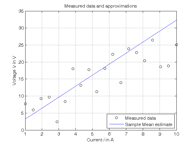
Estimation of the resistance using the Sample Mean algorithm
% Step 3: computation of the parameter estimate as mean of the R values
% derived from the Ohm's law for each couple of current-voltage data

R_SM = mean(V./i)   % Form #1: using the "mean" operator

R_SM_ = V'*(1./i)/N % Form #2: using the Sample Mean definition

% Step 4: graphical comparison of the results

V_SM = R_SM*i;
figure, plot(i,V,'ok', i,V_SM,'-b'),
axis([min(i),max(i),0,35]), grid, title('Measured data and approximations'),
xlabel('Current{\it i} in A'), ylabel('Voltage{\it V} in V'),
legend('Measured data','Sample Mean estimate',4)
R_SM =
    3.2324
R_SM_ =
    3.2324
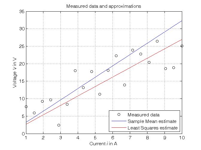
Estimation of the resistance using the Least Squares algorithm
% Step 5: computation of the parameter estimate

Phi=i;
R_LS=Phi\V   % Form #1: using the "\" operator (more realiable)

A=pinv(Phi); % more realiable than inv(Phi'*Phi)*Phi'
R_LS_=A*V    % Form #2: using the pseudoinverse matrix
sigma_e = 5;
Sigma_ee = sigma_e^2*eye(N);
Sigma_R_LS = pinv(Phi)*Sigma_ee*pinv(Phi)'

% Step 6: graphical comparison of the results

V_LS = R_LS*i;
figure, plot(i,V,'ok', i,V_SM,'-b', i,V_LS,'-r'),
axis([min(i),max(i),0,35]), grid, title('Measured data and approximations'),
xlabel('Current{\it i} in A'), ylabel('Voltage{\it V} in V'),
legend('Measured data','Sample Mean estimate','Least Squares estimate',4)
R_LS =
    2.6979
R_LS_ =
    2.6979
Sigma_R_LS =
    0.0331
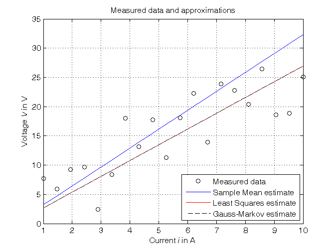
Estimation of the resistance using the Gauss-Markov algorithm
% Step 7: computation of the parameter estimate
% Note that the Gauss-Markov estimate coincides with the Least Squares
% estimate when the same weights are used for all the measurements

R_GM = inv(Phi'*inv(Sigma_ee)*Phi)*Phi'*inv(Sigma_ee)*V
Sigma_R_GM = inv(Phi'*inv(Sigma_ee)*Phi)

% Step 8: graphical comparison of the results

V_GM = R_GM*i;
figure, plot(i,V,'ok', i,V_SM,'-b', i,V_LS,'-r', i,V_GM,'--k'),
axis([min(i),max(i),0,35]), grid, title('Measured data and approximations'),
xlabel('Current{\it i} in A'), ylabel('Voltage{\it V} in V'),
legend('Measured data','Sample Mean estimate','Least Squares estimate',...
       'Gauss-Markov estimate',4)
R_GM =
    2.6979
Sigma_R_GM =
    0.0331
Estimation of the resistance using the Bayesian method
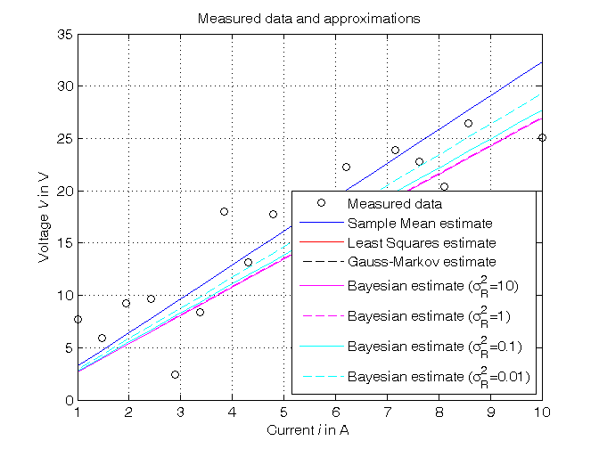
% Step 9: computation of the parameter estimate, assuming:
% - R_bar = a priori mean value of R = 3 (to be assumed early)
% - Sigma_RR = a priori variance of R = 10, 1, 0.1, 0.01 (to be assumed early)
% - V_bar = mean value of V = R_bar*i
% - Sigma_VV = Sigma_RR*i*i' + Sigma_ee
% - Sigma_RV = Sigma_RR*i'

R_bar = 3; % Try also with R_GM
Sigma_RR = [10, 1, 0.1, 0.01];
V_bar = R_bar*i;
for k=1:length(Sigma_RR),
    Sigma_VV = Sigma_RR(k)* i*i' + Sigma_ee;
    Sigma_RV = Sigma_RR(k)*i';
    R_B(k) = R_bar + Sigma_RV * inv(Sigma_VV) * (V-V_bar);
    Sigma_R_B(k) = Sigma_RV * inv(Sigma_VV) * Sigma_RV'; % estimate variance
    Sigma_R_minus_R_B(k) = Sigma_RR(k) - Sigma_R_B(k); % a posteriori variance
    V_B(:,k) = R_B(k)*i;
end
Sigma_RR, R_B, Sigma_R_B, Sigma_R_minus_R_B

% Step 10: graphical comparison of the results

figure, plot(i,V,'ok', i,V_SM,'-b', i,V_LS,'-r', i,V_GM,'--k', ...
             i,V_B(:,1),'-m', i,V_B(:,2),'--m', ...
             i,V_B(:,3),'-c', i,V_B(:,4),'--c'),
axis([min(i),max(i),0,35]), grid, title('Measured data and approximations'),
xlabel('Current{\it i} in A'), ylabel('Voltage{\it V} in V'),
legend('Measured data','Sample Mean estimate','Least Squares estimate',...
       'Gauss-Markov estimate', ...
       ['Bayesian estimate (\sigma_R^2=', num2str(Sigma_RR(1)),')'], ...
       ['Bayesian estimate (\sigma_R^2=', num2str(Sigma_RR(2)),')'], ...
       ['Bayesian estimate (\sigma_R^2=', num2str(Sigma_RR(3)),')'], ...
       ['Bayesian estimate (\sigma_R^2=', num2str(Sigma_RR(4)),')'],4)
Sigma_RR =
   10.0000    1.0000    0.1000    0.0100
R_B =
    2.6989    2.7076    2.7731    2.9300
Sigma_R_B =
    9.9670    0.9679    0.0751    0.0023
Sigma_R_minus_R_B =
    0.0330    0.0321    0.0249    0.0077