Laboratory 2 - Estimation, filtering and system identification - Prof. M. Taragna

Parametric estimation of a position transducer model using the Set Membership approach

Introduction
Procedure
Problem setup
Parametric estimation of a linear model (w.r.t. data) using least squares
Evaluation of estimate uncertainty intervals EUI in l-infinity norm
Evaluation of parameter uncertainty intervals PUI and central estimate in l-infinity norm
(Optional) Evaluation of an approximation of the feasible parameter set FPS

Introduction

The program code may be splitted in sections using the characters "%%". Each section can run separately with the command "Run Section" (in the Editor toolbar, just to the right of the "Run" button). You can do the same thing by highlighting the code you want to run and by using the button function 9 (F9). This way, you can run only the desired section of your code, saving your time. This script can be considered as a reference example.

clear all, close all, clc

Procedure

Load the file sensor.mat containing the position/voltage data
Plot the voltage measurements versus the position measurements
Estimate the parameters of the linear approximation using least squares
Plot the estimated approximation versus the experimental data
Compute the estimate uncertainty intervals EUI in l-infinity norm
Plot the EUI versus the estimated approximation
Compute the parameter uncertainty intervals PUI in l-infinity norm
Compute the parameter central estimate in l-infinity norm
Plot the PUI and the central estimate versus the experimental data
(Optional) Compute an approximation of the feasible parameter set FPS
(Optional) Plot PUI and FPS approximation versus the estimated parameters

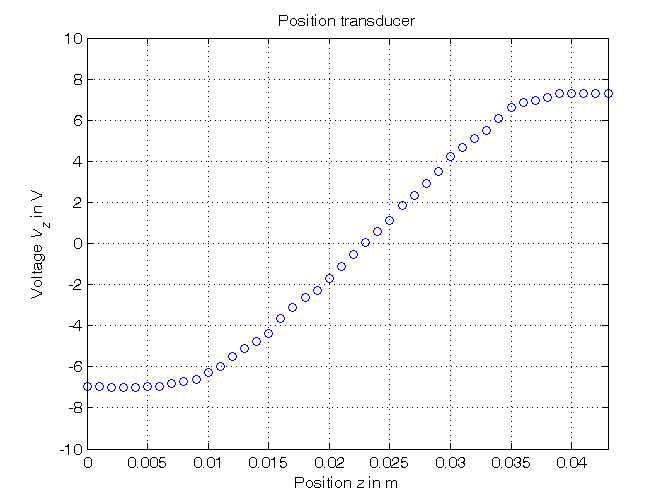
Problem setup

% Step 1: load of data

load sensor
% z  = position measured in meters, without position offset
% Vz = voltage measured in volts

% Step 2: plot of data

figure, plot(z,Vz,'o'),
axis([min(z),max(z),-10,10]), grid, title('Position transducer'),
xlabel('Position{\it z} in m'), ylabel('Voltage{\it V_z} in V')

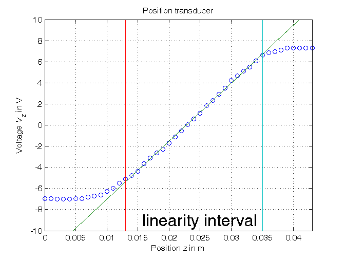
Parametric estimation of a linear model (w.r.t. data) using least squares

% Step3: computation of the parameter estimate

% definition of the linearity interval of the characteristic
i1=14; % z(11) = 0.01, z(14) = 0.013; use: i1=11 (at first), i1=14 (at the end)
i2=36; % z(36) = 0.035
z_lin=z(i1:i2);
Vz_lin=Vz(i1:i2);
N_lin=length(z_lin);

% parameter estimation by means of least squares algorithm
Phi=[Vz_lin, ones(N_lin,1)];
p=Phi\z_lin; % Form #1: using the "\" operator (more realiable)
Kt=1/p(1)
Vo=-p(2)/p(1)

A=pinv(Phi); % more realiable than inv(Phi'*Phi)*Phi'
p_=A*z_lin;  % Form #2: using the pseudoinverse matrix
Kt_=1/p_(1)
Vo_=-p_(2)/p_(1)

% Step 4: graphical comparison of the results

Vz0=linspace(-10,10,1000);
z_hat=p(1)*Vz0+p(2);
figure, plot(z,Vz,'o', z_hat,Vz0,'-', ...
             z_lin(1)*[1,1],[-10,10],'-', z_lin(end)*[1,1],[-10,10],'-'),
axis([min(z),max(z),-10,10]), grid, title('Position transducer'),
xlabel('Position{\it z} in m'), ylabel('Voltage{\it V_z} in V'),
text(0.015,-9,'\fontsize{20} linearity interval')

Kt =
  549.6215
Vo =
  -12.5263
Kt_ =
  549.6215
Vo_ =
  -12.5263

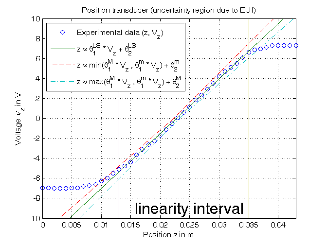
Evaluation of estimate uncertainty intervals EUI in l-infinity norm

% Step 5: computation of the estimate uncertainty intervals EUI in l-infinity norm

% bound on the greatest measurement error of the position z
format compact, format short e
epsilon=0.5e-3

% EUI algorithm in compact form
for ind=1:length(p),
    p_min(ind,1)=A(ind,:)*(z_lin-epsilon*sign(A(ind,:))');
end
p_max=2*p-p_min;
EUI=[p_min, p_max]

% EUI algorithm in extended form, using a loop (equivalent)
p_min_=zeros(size(p)); ; p_max_=zeros(size(p));
for k=1:length(A),
    p_min_(1)=p_min_(1)+A(1,k)*(z_lin(k)-epsilon*sign(A(1,k)));
    p_min_(2)=p_min_(2)+A(2,k)*(z_lin(k)-epsilon*sign(A(2,k)));
    p_max_(1)=p_max_(1)+A(1,k)*(z_lin(k)+epsilon*sign(A(1,k)));
    p_max_(2)=p_max_(2)+A(2,k)*(z_lin(k)+epsilon*sign(A(2,k)));
end
EUI_=[p_min_, p_max_]

format compact, format short
Kt_min=1/p_max(1)
Kt_max=1/p_min(1)
Vo_min=-p_max(2)/p_min(1)
Vo_max=-p_min(2)/p_max(1)

% Step 6: graphical comparison of the results

z_min=min([p_max(1)*Vz0; p_min(1)*Vz0])+p_min(2);
z_max=max([p_max(1)*Vz0; p_min(1)*Vz0])+p_max(2);

figure, plot(z,Vz,'o', z_hat,Vz0,'-', ...
             z_min,Vz0,'--', z_max,Vz0,'-.', ...
             z_lin(1)*[1,1],[-10,10],'-',z_lin(end)*[1,1],[-10,10],'-')
axis([min(z),max(z),-10,10]), grid,
title('Position transducer (uncertainty region due to EUI)'),
xlabel('Position{\it z} in m'), ylabel('Voltage{\it V_z} in V'),
legend('Experimental data (z, V_z)_{ }^{  }', ...
       'z \approx \theta_{1}^{LS} * V_{z} + \theta_2^{LS}', ...
       'z \approx min(\theta_{1}^{M} * V_{z} , \theta_{1}^{m} * V_{z}) + \theta_{2}^{m}', ...
       'z \approx max(\theta_{1}^{M} * V_{z} , \theta_{1}^{m} * V_{z}) + \theta_{2}^{M}', 2),
text(0.015,-9,'\fontsize{20} linearity interval')

epsilon =
   5.0000e-04
EUI =
   1.6996e-03   1.9392e-03
   2.2291e-02   2.3291e-02
EUI_ =
   1.6996e-03   1.9392e-03
   2.2291e-02   2.3291e-02
Kt_min =
  515.6654
Kt_max =
  588.3648
Vo_min =
  -13.7035
Vo_max =
  -11.4946

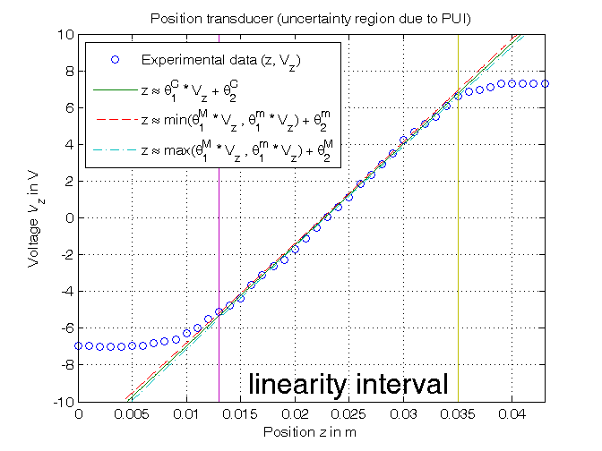
Evaluation of parameter uncertainty intervals PUI and central estimate in l-infinity norm

% Step 7: computation of the parameter uncertainty intervals PUI in l-infinity norm

% PUI_LP(1,1)=[1;0]'*lp( [1;0],[Phi;-Phi],[z_lin+epsilon;-z_lin+epsilon]); % Under Matlab 5.3
% PUI_LP(2,1)=[0;1]'*lp( [0;1],[Phi;-Phi],[z_lin+epsilon;-z_lin+epsilon]); % Under Matlab 5.3
% PUI_LP(1,2)=[1;0]'*lp(-[1;0],[Phi;-Phi],[z_lin+epsilon;-z_lin+epsilon]); % Under Matlab 5.3
% PUI_LP(2,2)=[0;1]'*lp(-[0;1],[Phi;-Phi],[z_lin+epsilon;-z_lin+epsilon]); % Under Matlab 5.3

options_old=optimset('linprog'); % default value for 'Algorithm' option is 'interior-point'
options_new=optimset(options_old, 'Algorithm','simplex');
PUI(1,1)=[1; 0]'*linprog( [1; 0],[Phi; -Phi],[z_lin+epsilon; -z_lin+epsilon], ...
                          [],[],[],[],[],options_new);
PUI(2,1)=[0; 1]'*linprog( [0; 1],[Phi; -Phi],[z_lin+epsilon; -z_lin+epsilon], ...
                          [],[],[],[],[],options_new);
PUI(1,2)=[1; 0]'*linprog(-[1; 0],[Phi; -Phi],[z_lin+epsilon; -z_lin+epsilon], ...
                          [],[],[],[],[],options_new);
PUI(2,2)=[0; 1]'*linprog(-[0; 1],[Phi; -Phi],[z_lin+epsilon; -z_lin+epsilon], ...
                          [],[],[],[],[],options_new);

format compact, format short e
PUI

format compact, format short
Kt_min_PUI=1/PUI(1,2)
Kt_max_PUI=1/PUI(1,1)
Vo_min_PUI=-PUI(2,2)/PUI(1,1)
Vo_max_PUI=-PUI(2,1)/PUI(1,2)

% Step 8: computation of the central estimate

format compact, format short e
p_central=[(PUI(1,1)+PUI(1,2))/2; (PUI(2,1)+PUI(2,2))/2]

format compact, format short
Kt_central=1/p_central(1)
Vo_central=-p_central(2)/p_central(1)

% Step 9: graphical comparison of the results

z_hat_central=p_central(1)*Vz0+p_central(2);
z_min_central=min([PUI(1,2)*Vz0; PUI(1,1)*Vz0])+PUI(2,1);
z_max_central=max([PUI(1,2)*Vz0; PUI(1,1)*Vz0])+PUI(2,2);

figure, plot(z,Vz,'o', z_hat_central,Vz0,'-', ...
             z_min_central,Vz0,'--', z_max_central,Vz0,'-.', ...
             z_lin(1)*[1,1],[-10,10],'-',z_lin(end)*[1,1],[-10,10],'-')
axis([min(z),max(z),-10,10]), grid,
title('Position transducer (uncertainty region due to PUI)'),
xlabel('Position{\it z} in m'), ylabel('Voltage{\it V_z} in V'),
legend('Experimental data (z, V_z)_{ }^{  }', ...
       'z \approx \theta_{1}^{C} * V_{z} + \theta_2^{C}', ...
       'z \approx min(\theta_{1}^{M} * V_{z} , \theta_{1}^{m} * V_{z}) + \theta_{2}^{m}', ...
       'z \approx max(\theta_{1}^{M} * V_{z} , \theta_{1}^{m} * V_{z}) + \theta_{2}^{M}', 2),
text(0.015,-9,'\fontsize{20} linearity interval')

Optimization terminated.
Optimization terminated.
Optimization terminated.
Optimization terminated.
PUI =
   1.7909e-03   1.8484e-03
   2.2596e-02   2.2807e-02
Kt_min_PUI =
  541.0083
Kt_max_PUI =
  558.3842
Vo_min_PUI =
  -12.7353
Vo_max_PUI =
  -12.2246
p_central =
   1.8196e-03
   2.2702e-02
Kt_central =
  549.5590
Vo_central =
  -12.4759

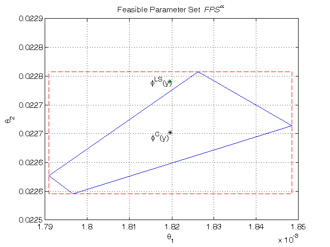
(Optional) Evaluation of an approximation of the feasible parameter set FPS

% Step 10: computation of a polytopic outer approximation of the FPS

n=16; % Number of vertices of the polytope
theta_vect=[];
for k=0:n-1,
    theta=linprog([sin(2*pi*k/n),cos(2*pi*k/n)],[Phi;-Phi],[z_lin+epsilon;-z_lin+epsilon], ...
                  [],[],[],[],[],options_new);
    theta_vect=[theta_vect, theta];
end

% Step 11: graphical comparison of the results

k=convhull(theta_vect(1,:),theta_vect(2,:));
figure, plot(theta_vect(1,k),theta_vect(2,k),'-',p(1),p(2),'*', ...
   [PUI(1,1),PUI(1,:),PUI(1,2:-1:1)], [PUI(2,2:-1:1),PUI(2,:),PUI(2,2)],'--', ...
   p_central(1),p_central(2),'*k'),
grid on, text(p(1)*0.9975,p(2),'\phi^{LS}(y)'),
text(p_central(1)*0.9975,p_central(2)*0.9997,'\phi^{C}(y)'),
title('Feasible Parameter Set {\it FPS^\infty}'),
xlabel('\theta_{1}'), ylabel('\theta_{2}')

Optimization terminated.
Optimization terminated.
Optimization terminated.
Optimization terminated.
Optimization terminated.
Optimization terminated.
Optimization terminated.
Optimization terminated.
Optimization terminated.
Optimization terminated.
Optimization terminated.
Optimization terminated.
Optimization terminated.
Optimization terminated.
Optimization terminated.
Optimization terminated.