Laboratory 1 - Estimation, filtering and system identification - Prof. M. Taragna

Parametric estimation of position transducer models using the classical (or statistical) approach

Introduction
Procedure
Problem setup
Parametric estimation of a linear model (w.r.t. data) using least squares
Computation of the parameter confidence intervals (noise variance derived from priors)
Computation of the parameter confidence intervals (noise variance estimated from data)
Parametric estimation of 3rd order polynomial models (w.r.t. data) using least squares

Introduction

The program code may be splitted in sections using the characters "%%". Each section can run separately with the command "Run Section" (in the Editor toolbar, just to the right of the "Run" button). You can do the same thing by highlighting the code you want to run and by using the button function 9 (F9). This way, you can run only the desired section of your code, saving your time. This script can be considered as a reference example.

clear all, close all, clc

Procedure

Load the file sensor.mat containing the position/voltage data
Plot the voltage measurements versus the position measurements
Estimate the parameters of the linear approximation using least squares
Plot the estimated approximation versus the experimental data
Evaluate the estimate uncertaity using the prior information only
Plot these confidence intervals versus the estimated approximation
Evaluate the estimate uncertaity using the experimental data only
Plot these confidence intervals versus the estimated approximation
Estimate the parameters of polynomial approximations using least squares
Plot the estimated approximations versus the experimental data

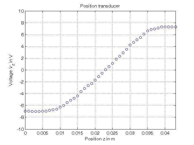
Problem setup

% Step 1: load of data

load sensor
% z  = position measured in meters, without position offset
% Vz = voltage measured in volts

% Step 2: plot of data

figure, plot(z,Vz,'o'),
axis([min(z),max(z),-10,10]), grid, title('Position transducer'),
xlabel('Position{\it z} in m'), ylabel('Voltage{\it V_z} in V')

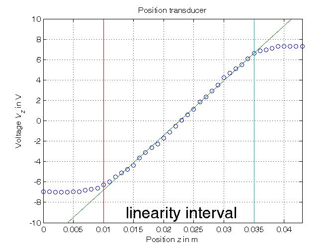
Parametric estimation of a linear model (w.r.t. data) using least squares

% Step3: computation of the parameter estimate

% definition of the linearity interval of the characteristic
i1=11; % z(11) = 0.01
i2=36; % z(36) = 0.035
z_lin=z(i1:i2);
Vz_lin=Vz(i1:i2);
N_lin=length(z_lin);

% parameter estimation by means of least squares algorithm
Phi=[Vz_lin, ones(N_lin,1)];
p=Phi\z_lin; % Form #1: using the "\" operator (more realiable)
Kt=1/p(1)
Vo=-p(2)/p(1)

p_=inv(Phi'*Phi)*Phi'*z_lin; % Form #2: using the pseudoinverse matrix
Kt_=1/p_(1)
Vo_=-p_(2)/p_(1)

% Step 4: graphical comparison of the results

Vz0=linspace(-10,10,1000);
z_hat=p(1)*Vz0+p(2);
figure, plot(z,Vz,'o', z_hat,Vz0,'-', ...
             z_lin(1)*[1,1],[-10,10],'-', z_lin(end)*[1,1],[-10,10],'-'),
axis([min(z),max(z),-10,10]), grid, title('Position transducer'),
xlabel('Position{\it z} in m'), ylabel('Voltage{\it V_z} in V'),
text(0.013,-9,'\fontsize{20} linearity interval')

Kt =
  537.0036
Vo =
  -12.1779
Kt_ =
  537.0036
Vo_ =
  -12.1779

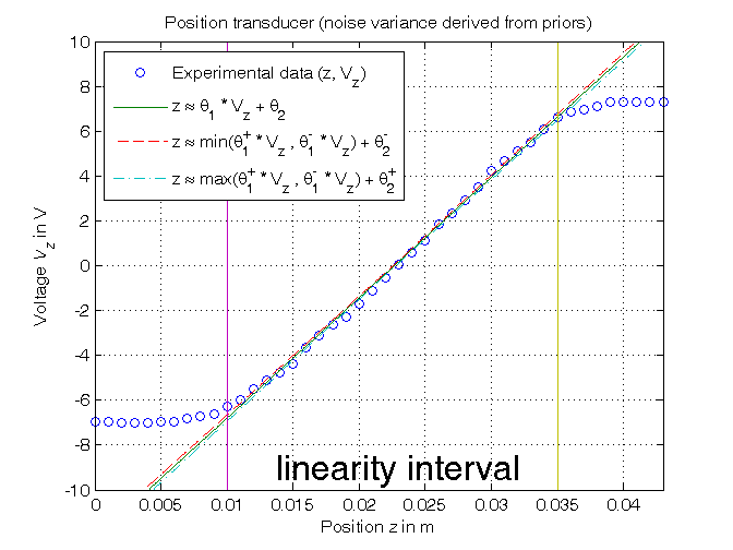
Computation of the parameter confidence intervals (noise variance derived from priors)

% Step 5: computation of the confidence intervals

% Definition of the x% confidence intervals:
% x=95.4 => k=2 ("2 sigma"); x=99.7 => k=3 ("3 sigma")
k_e=2; k_p=2;
noise_max=5e-4;

sigma_e=noise_max/k_e

Sigma_e=sigma_e^2*eye(N_lin);
Sigma_p=inv(Phi'*inv(Sigma_e)*Phi);
sigma_p=sqrt(diag(Sigma_p));
delta_p=k_p*sigma_p;
p_min=p-delta_p;
p_max=p+delta_p;
Kt_min=1/p_max(1)
Kt_max=1/p_min(1)
Vo_min=-p_max(2)/p_min(1)
Vo_max=-p_min(2)/p_max(1)

% Step 6: graphical comparison of the results

z_min=min([p_max(1)*Vz0; p_min(1)*Vz0])+p_min(2);
z_max=max([p_max(1)*Vz0; p_min(1)*Vz0])+p_max(2);

figure, plot(z,Vz,'o', z_hat,Vz0,'-', ...
             z_min,Vz0,'--', z_max,Vz0,'-.', ...
             z_lin(1)*[1,1],[-10,10],'-',z_lin(end)*[1,1],[-10,10],'-')
axis([min(z),max(z),-10,10]), grid,
title('Position transducer (noise variance derived from priors)'),
xlabel('Position{\it z} in m'), ylabel('Voltage{\it V_z} in V'),
legend('Experimental data (z, V_z)_{ }^{  }', ...
       'z \approx \theta_{1} * V_{z} + \theta_2', ...
       'z \approx min(\theta_{1}^{+} * V_{z} , \theta_{1}^{-} * V_{z}) + \theta_{2}^{-}', ...
       'z \approx max(\theta_{1}^{+} * V_{z} , \theta_{1}^{-} * V_{z}) + \theta_{2}^{+}', 2),
text(0.013,-9,'\fontsize{20} linearity interval')

sigma_e =
   2.5000e-04
Kt_min =
  530.0654
Kt_max =
  544.1257
Vo_min =
  -12.3928
Vo_max =
  -11.9685

Computation of the parameter confidence intervals (noise variance estimated from data)

% Step 7: computation of the confidence intervals

sigma_e_ml=sqrt((z_lin-Phi*p)'*(z_lin-Phi*p)/N_lin)

Sigma_e=sigma_e_ml^2*eye(N_lin);
Sigma_p=inv(Phi'*inv(Sigma_e)*Phi);
sigma_p=sqrt(diag(Sigma_p));
delta_p=k_p*sigma_p;
p_min=p-delta_p;
p_max=p+delta_p;
Kt_min=1/p_max(1)
Kt_max=1/p_min(1)
Vo_min=-p_max(2)/p_min(1)
Vo_max=-p_min(2)/p_max(1)

% Step 8: graphical comparison of the results

z_min=min([p_max(1)*Vz0; p_min(1)*Vz0])+p_min(2);
z_max=max([p_max(1)*Vz0; p_min(1)*Vz0])+p_max(2);

figure, plot(z,Vz,'o', z_hat,Vz0,'-', ...
             z_min,Vz0,'--', z_max,Vz0,'-.', ...
             z_lin(1)*[1,1],[-10,10],'-',z_lin(end)*[1,1],[-10,10],'-')
axis([min(z),max(z),-10,10]), grid,
title('Position transducer (noise variance estimated from data)'),
xlabel('Position{\it z} in m'), ylabel('Voltage{\it V_z} in V'),
legend('Experimental data (z, V_z)_{ }^{  }', ...
       'z \approx \theta_{1} * V_{z} + \theta_2', ...
       'z \approx min(\theta_{1}^{+} * V_{z} , \theta_{1}^{-} * V_{z}) + \theta_{2}^{-}', ...
       'z \approx max(\theta_{1}^{+} * V_{z} , \theta_{1}^{-} * V_{z}) + \theta_{2}^{+}', 2),
text(0.013,-9,'\fontsize{20} linearity interval')

sigma_e_ml =
   3.5618e-04
Kt_min =
  527.1726
Kt_max =
  547.2082
Vo_min =
  -12.4858
Vo_max =
  -11.8813

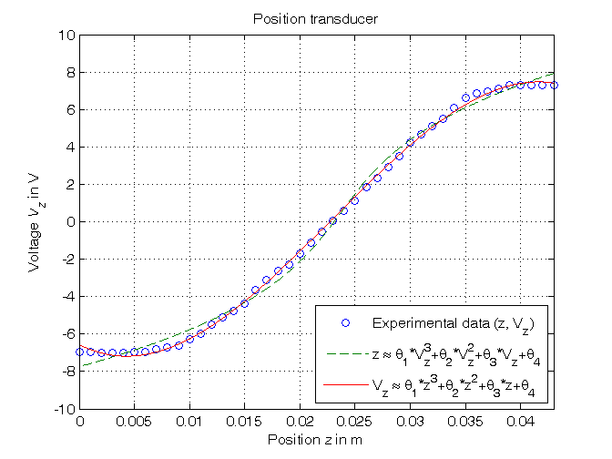
Parametric estimation of 3rd order polynomial models (w.r.t. data) using least squares

% Step 9: computation of the parameter estimate

% a) assuming Vz as independent variable, z as variable dependent on Vz =>
%    z = theta(1)*Vz^3 + theta(2)*Vz^2 + theta(3)*Vz + theta(4)
Phi=[Vz.^3, Vz.^2, Vz, Vz.^0];
format shortE, format compact
p3a=Phi\z                      % Form #1: using the "\" operator
z_pol=polyval(p3a,Vz0);

p3a_=polyfit(Vz,z,3)           % Form #2: using the "polyfit" function
format short, format compact

% b) assuming z as independent variable, Vz as variable dependent on z =>
%    Vz = theta(1)*z^3 + theta(2)*z^2 + theta(3)*z + theta(4)
Phi=[z.^3, z.^2, z, z.^0];
p3b=Phi\Vz                     % Form #1: using the "\" operator
z0=linspace(min(z),max(z),1000);
Vz_pol=polyval(p3b,z0);

p3b_=polyfit(z,Vz,3)           % Form #2: using the "polyfit" function

% Step 10: graphical comparison of the results

figure, plot(z,Vz,'o',z_pol,Vz0,'--',z0,Vz_pol,'-'),
axis([min(z),max(z),-10,10]), grid, title('Position transducer'),
xlabel('Position{\it z} in m'), ylabel('Voltage{\it V_z} in V'),
legend('Experimental data (z, V_z)_{ }^{  }', ...
       'z \approx \theta_1*V_z^3+\theta_2*V_z^2+\theta_3*V_z+\theta_4', ...
       'V_z \approx \theta_1*z^3+\theta_2*z^2+\theta_3*z+\theta_4',4)

p3a =
   2.4097e-05
  -3.4590e-05
   1.2715e-03
   2.3100e-02
p3a_ =
   2.4097e-05  -3.4590e-05   1.2715e-03   2.3100e-02
p3b =
   1.0e+05 *
   -5.6269
    0.3877
   -0.0030
   -0.0001
p3b_ =
   1.0e+05 *
   -5.6269    0.3877   -0.0030   -0.0001